🙇🏾 📃 🧗 わいせつなアプリケーション 🔸 🤪 👩🏽‍💼

記事への添付では、粒子の経路、切り取られた材料が提供されています。経路積分、ネオンの冷たい原子の二重スリット実験、粒子テレポーテーションのフレーム、および残酷で性的な性質のその他のシーンです。

私の意見では、その結果が経験から逸脱していることを実証するか、その予測が観察の可能性を使い果たしていないことを証明する以外に、数学的形式を論理的に一貫していると見なす方法はありません。

ニールスボーア

結論として、著者は、広範な現象を説明する理論を拒否する2つの正当な理由のみを認めると述べたいと思います。第一に、理論は内部的に一貫しておらず、第二に、それは実験と一致していません。

デビッドボーム

以前の私たちは学んだ、それがそこから取られている理由シュレディンガー方程式は、どこから来るか、そしてどのようにそれは、種々の方法で取られます

i ℏ \frac{\partial Ψ}{\partial t} = (- \frac{ℏ^{2}}{2 m} \nabla^{2} + V) Ψ

$i\hbar\frac{\partial\Psi}{\partial t} = \left( -\frac{\hbar^2}{2m}\nabla^2 + V\right) \Psi$

ここで、2つの実際の方程式に分解します。これを行うには、psiを極形式で表します $\Psi = Re^{iS/\hbar}$ , :

\frac{\partial S}{\partial t} + \frac{(\nabla S)^{2}}{2 m} - \frac{ℏ^{2}}{2 m} \frac{\nabla^{2} R}{R} + V = 0 \frac{\partial R^{2}}{\partial t} + \nabla \cdot (\frac{R^{2} \nabla S}{m}) = 0

$\frac{\partial S}{\partial t}+\frac{(\nabla S)^{2}}{2 m}-\frac{\hbar^{2}}{2 m} \frac{\nabla^{2} R}{R}+V=0 \\ \frac{\partial R^{2}}{\partial t}+\nabla \cdot\left(\frac{R^{2} \nabla S}{m}\right)=0$

S — , R — . , , , — -, ( ).

, $U = \nabla S /m$ . , S -, - - :

S = - \frac{i ℏ}{2} \ln \frac{Ψ}{Ψ^{*}}

$S = -\frac{i\hbar}{2}\ln\frac{\Psi}{\Psi^*}$

, -, , , , S, , , , . , , . -.

— , . , , , . , , , .

, , , . . . , , , .

, .

, , , . , ( - ). :

()

, , , : ,

, . . .

U = \nabla S / m = - \frac{i ℏ}{2 m} \nabla \ln \frac{Ψ}{Ψ^{*}} = \frac{ℏ}{m} I m (\frac{\nabla ψ}{ψ})

$U = \nabla S /m = -\frac{i\hbar}{2m}\nabla\ln\frac{\Psi}{\Psi^*} = \frac{\hbar}{m}\mathrm{Im}\left(\frac{\nabla\psi}{\psi} \right)$

-, :

x + = U Δ t

$x += U\Delta t$

using LinearAlgebra, SparseArrays, Plots

const ħ = 1.0546e-34 # J*s
const m = 9.1094e-31 # kg
const q = 1.6022e-19 # Kl
const nm = 1e-9 # m
const fs = 1e-12; # s

function wavefun()

    gauss(x) = exp( -(x-x0)^2 / (2*σ^2) + im*x*k )
    k = m*v/ħ

    #    
    Vm = spdiagm(0 => V )
    H = spdiagm(-1 => ones(Nx-1), 0 => -2ones(Nx), 1 => ones(Nx-1) )
    H *= ħ^2 / ( 2m*dx^2 )
    H += Vm

    A = I + 0.5im*dt/ħ * H #  
    B = I - 0.5im*dt/ħ * H # 
    psi = zeros(Complex, Nx, Nt)
    psi[:,1] = gauss.(x)

    for t = 1:Nt-1

        b = B * psi[:,t]
        #       A*psi = b
        psi[:,t+1] = A \ b
    end

    return psi
end

dx = 0.05nm # x step
dt = 0.01fs # t step
xlast = 400nm
Nt = 260 # Number of time steps
t = range(0, length = Nt, step = dt)

x = [0:dx:xlast;]
Nx = length(x) # Number of spatial steps

a1 = 200nm
a2 = 200.5nm # 5 
a3 = 205nm
a4 = 205.5nm 
#V = [ a1<xi<a2 ? 2q : 0.0 for xi in x ] # 2 eV 
V = [ a1<xi<a2 || a3<xi<a4 ? 2q : 0.0 for xi in x ] # 2 eV 

x0 = 80nm # Initial position
σ = 20nm # gauss width
v = -120nm/fs;

@time Psi = wavefun()
P = abs2.(Psi);

function ψ(xi, j)

    k = findfirst(el-> abs(el-xi)<dx, x)
    k == nothing && ( k = 1 )

    Psi[k, j]
end

function corpusculaz(n)

    X = zeros(n, Nt)
    X[:,1] = x0 .+ σ*randn(n)

    for j in 2:Nt, i in 1:n
        U = ħ/(2m*dx) * imag( ( ψ(X[i,j-1]+dx, j) -  ψ(X[i,j-1]-dx, j) ) /  ψ(X[i,j-1], j) )
        X[i,j] = X[i,j-1] - U*dt
    end

    X
end

@time X = corpusculaz(20);

plot(x, P[:, 1], legend = false)
plot!(x, P[:, 80], legend = false)
scatter!( X[:,1], zeros(20) )
scatter!( X[:,80], zeros(20) )

. — , . :

, . , , !

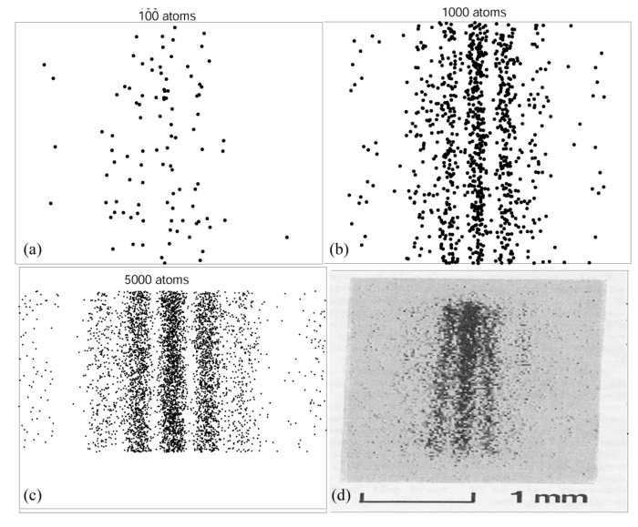
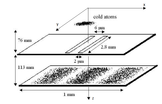
, . Double-slit interference with ultracold metastable neon atoms — - .

using Random, Gnuplot, Statistics
#  
function trapez(f, a, b, n)
    h = (b - a)/n
    result = 0.5*(f(a) + f(b))
    for i in 1:n-1
        result += f(a + i*h)
    end
    result * h
end
#  
function rk4(f, x, y, h)
    k1 = h * f(x       , y        )
    k2 = h * f(x + 0.5h, y + 0.5k1)
    k3 = h * f(x + 0.5h, y + 0.5k2)
    k4 = h * f(x +    h, y +    k3)

    return y + (k1 + 2*(k2 + k3) + k4)/6.0
end

const ħ = 1.055e-34 # J*s 
const kB = 1.381e-23 # J*K-1
const g = 9.8 # m/s^2

const l1 = 76e-3 # m
const l2 = 113e-3 # m
const yh = 2.8e-3 # m
const d = 6e-6 # m
const b = 2e-6 # m
const a1 = 0.5(- d - b) # 
const a2 = 0.5(- d + b)
const b1 = 0.5(  d - b)
const b2 = 0.5(  d + b)

const m = 3.349e-26 # kg
const T = 2.5e-3 # K
const σv = sqrt(kB*T/m) #  
const σ₀ = 10e-6 # 10 mkm #      
const σz = 3e-4 # 0.3 mm #  z
const σk = m*σv / (ħ*√3) # 2e8 m/s #    

v₀ = zeros(3)
k₀ = zeros(3);

: , , -, .

\begin{aligned} 1) ψ_{0} (x, y, z; k_{0 x}, k_{0 y}, k_{0 z}) = & ψ_{0 x} (x; k_{0 x}) ψ_{0_{y}} (z; k_{0 y}) ψ_{0 z} (z; k_{0 z}) \\ = & {(2 π σ_{0}^{2})}^{- 1 / 4} e^{- x^{2} / 4 σ_{0}^{2}} e^{i k_{0 x} x} \\ \times {(2 π σ_{0}^{2})}^{- 1 / 4} e^{- y^{2} / 4 σ_{0}^{2}} e^{i k_{0 y} y} \\ \times {(2 π σ_{z}^{2})}^{- 1 / 4} e^{- z^{2} / 4 σ_{z}^{2}} e^{i k_{0 z} z} \end{aligned}

$\begin{aligned} 1)\psi_{0}\left(x, y, z ; k_{0 x}, k_{0 y}, k_{0 z}\right)=& \psi_{0 x}\left(x ; k_{0 x}\right) \psi_{0_{y}}\left(z ; k_{0 y}\right) \psi_{0 z}\left(z ; k_{0 z}\right) \\ =&\left(2 \pi \sigma_{0}^{2}\right)^{-1 / 4} e^{-x^{2} / 4 \sigma_{0}^{2}} e^{i k_{0 x} x} \\ & \times\left(2 \pi \sigma_{0}^{2}\right)^{-1 / 4} e^{-y^{2} / 4 \sigma_{0}^{2}} e^{i k_{0 y} y} \\ & \times\left(2 \pi \sigma_{z}^{2}\right)^{-1 / 4} e^{-z^{2} / 4 \sigma_{z}^{2}} e^{i k_{0 z} z} \end{aligned}$

, . , , , . , , .

, . , , — . , , , . , , .

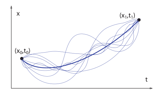
Quantum Mechanics And Path Integrals, A. R. Hibbs, R. P. Feynman, , 3.6 .

K (β, t_{β}; α, t_{α}) = K_{x} (x_{β}, t_{β}; x_{α}, t_{α}) K_{y} (y_{β}, t_{β}; y_{α}, t_{α}) K_{z} (z_{β}, t_{β}; z_{α}, t_{α})

$K\left(\beta, t_{\beta} ; \alpha, t_{\alpha}\right)=K_{x}\left(x_{\beta}, t_{\beta} ; x_{\alpha}, t_{\alpha}\right) K_{y}\left(y_{\beta}, t_{\beta} ; y_{\alpha}, t_{\alpha}\right) K_{z}\left(z_{\beta}, t_{\beta} ; z_{\alpha}, t_{\alpha}\right)$

\begin{aligned} K_{x} (x_{β}, t_{β}; x_{α}, t_{α}) = & {(\frac{m}{2 i π ℏ (t_{β} - t_{α})})}^{1 / 2} \exp \frac{i m}{ℏ} (\frac{{(x_{β} - x_{α})}^{2}}{2 (t_{β} - t_{α})}) \\ K_{y} (y_{β}, t_{β}; y_{α}, t_{α}) = & {(\frac{m}{2 i π ℏ (t_{β} - t_{α})})}^{1 / 2} \exp \frac{i m}{ℏ} (\frac{{(y_{β} - y_{α})}^{2}}{2 (t_{β} - t_{α})}) \\ K_{z} (z_{β}, t_{β}; z_{α}, t_{α}) = & {(\frac{m}{2 i π ℏ (t_{β} - t_{α})})}^{1 / 2} \exp \frac{i m}{ℏ} (\frac{{(z_{β} - z_{α})}^{2}}{2 (t_{β} - t_{α})}) \\ \times \exp \frac{i m}{ℏ} (\frac{g}{2} (z_{β} + z_{α}) (t_{β} - t_{α}) - \frac{g^{2}}{24} {(t_{β} - t_{α})}^{3}) \end{aligned}

$\begin{aligned} K_{x}\left(x_{\beta}, t_{\beta} ; x_{\alpha}, t_{\alpha}\right)=&\left(\frac{m}{2 i \pi \hbar\left(t_{\beta}-t_{\alpha}\right)}\right)^{1 / 2} \exp \frac{i m}{\hbar}\left(\frac{\left(x_{\beta}-x_{\alpha}\right)^{2}}{2\left(t_{\beta}-t_{\alpha}\right)}\right) \\ K_{y}\left(y_{\beta}, t_{\beta} ; y_{\alpha}, t_{\alpha}\right)=&\left(\frac{m}{2 i \pi \hbar\left(t_{\beta}-t_{\alpha}\right)}\right)^{1 / 2} \exp \frac{i m}{\hbar}\left(\frac{\left(y_{\beta}-y_{\alpha}\right)^{2}}{2\left(t_{\beta}-t_{\alpha}\right)}\right) \\ K_{z}\left(z_{\beta}, t_{\beta} ; z_{\alpha}, t_{\alpha}\right)=&\left(\frac{m}{2 i \pi \hbar\left(t_{\beta}-t_{\alpha}\right)}\right)^{1 / 2} \exp \frac{i m}{\hbar}\left(\frac{\left(z_{\beta}-z_{\alpha}\right)^{2}}{2\left(t_{\beta}-t_{\alpha}\right)}\right) \\ & \times \exp \frac{i m}{\hbar}\left(\frac{g}{2}\left(z_{\beta}+z_{\alpha}\right)\left(t_{\beta}-t_{\alpha}\right)-\frac{g^{2}}{24}\left(t_{\beta}-t_{\alpha}\right)^{3}\right) \end{aligned}$

Z , . ,

ψ (β, t) = \int K (β, t; α, t_{α}) ψ (α, t_{α}) d x_{α}, d y_{α}, d z_{α}

$\psi\left(\beta, t \right)=\int K\left(\beta, t ; \alpha, t_{\alpha}\right) \psi\left(\alpha, t_{\alpha}\right) d x_{\alpha}, d y_{\alpha}, d z_{\alpha}$

, . , X, . :

\begin{aligned} ψ_{x} (x, t; k_{0 x}) & = \int K (x, t; x_{α}, 0) ψ_{0} (x_{α}) d x_{α} \\ ψ_{x} (x, t; k_{0 x}) & = {(2 π s_{0}^{2} (t))}^{- 1 / 4} \exp [- \frac{{(x - v_{0 x} t)}^{2}}{4 σ_{0} s_{0} (t)} + i k_{0 x} (x - v_{0 x} t)] \\ ρ_{x} (x, t) & = {(2 π ε_{0}^{2} (t))}^{- 1 / 2} \exp [- \frac{x^{2}}{2 ε_{0}^{2} (t)}] \end{aligned}

$\begin{aligned} \psi_{x}\left(x, t ; k_{0 x}\right)&=\int K\left(x, t ; x_\alpha, 0\right) \psi_0\left(x_\alpha\right) d x_{\alpha}\\ \psi_{x}\left(x, t ; k_{0 x}\right) &=\left(2 \pi s_{0}^{2}(t)\right)^{-1 / 4} \exp \left[-\frac{\left(x-v_{0 x} t\right)^{2}}{4 \sigma_{0} s_{0}(t)}+i k_{0 x}\left(x-v_{0 x} t\right)\right] \\ \rho_{x}(x, t) &=\left(2 \pi \varepsilon_{0}^{2}(t)\right)^{-1 / 2} \exp \left[-\frac{x^{2}}{2 \varepsilon_{0}^{2}(t)}\right] \end{aligned}$

ε_{0}^{2} (t) = σ_{0}^{2} (t) + {(\frac{h t σ_{v}}{m})}^{2} σ_{0}^{2} (t) = σ_{0}^{2} + {(\frac{h t}{2 m σ_{0}^{2}})}^{2}

$\varepsilon_{0}^{2}(t)=\sigma_{0}^{2}(t)+\left(\frac{h t \sigma_v}{m}\right)^{2}\\ \sigma_{0}^{2}(t)=\sigma_{0}^{2}+\left(\frac{h t}{2 m \sigma_{0}^{2}}\right)^{2}$

, :

ε₀(t) = σ₀^2 + ( ħ/(2m*σ₀) * t )^2 + (ħ*t*σv/m)^2
s₀(t) = σ₀ + im*ħ/(2m*σ₀) * t

ρₓ(x, t) = exp( -x^2 / (2ε₀(t)) ) / sqrt( 2π*ε₀(t) )

t₁(v, z) = sqrt( 2*(l1-z)/g + (v/g)^2 ) - v/g
tf1 = t₁(v₀[3], 0) # s #    
X1 = range(-100, stop = 100, length = 100)*1e-6 
Z1 = range(0, stop = l1, length = 100)
Cron1 = range(0, stop = tf1, length = 100)

P1 = [ ρₓ(x, t) for t in Cron1, x in X1 ]
P1 /= maximum(P1); #   

@gp "set title 'Wavefun before the slits'" xlab="Z, mkm" ylab="X, mkm"
@gp :- 1000Z1 1000000X1 P1 "w image notit"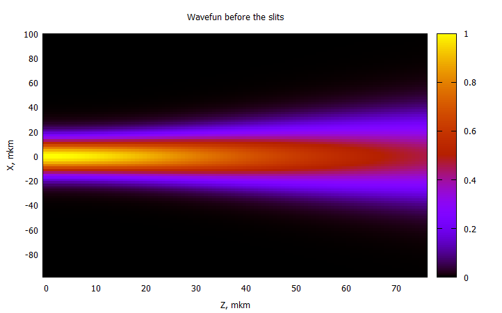

— .

, :

\begin{aligned} ψ_{x} & (x, t) = ψ_{A} + ψ_{B} \\ ψ_{A} & = \int_{A} K_{x} (x, t; x_{a}, t_{1}) ψ_{x} (x_{a}, t_{1}, k_{0 x}) d x_{a} \\ ψ_{B} & = \int_{B} K_{x} (x, t; x_{b}, t_{1}) ψ_{x} (x_{b}, t_{1}, k_{0 x}) d x_{b} \end{aligned}

$\begin{aligned} \psi_{x}&\left(x, t\right)=\psi_{A}+\psi_{B}\\ \psi_{A} &=\int_{A} K_{x}\left(x, t ; x_{a}, t_{1}\right) \psi_{x}\left(x_{a}, t_{1}, k_{0 x}\right) d x_{a} \\ \psi_{B} &=\int_{B} K_{x}\left(x, t ; x_{b}, t_{1}\right) \psi_{x}\left(x_{b}, t_{1}, k_{0 x}\right) d x_{b} \end{aligned}$

ρ_{x} (x, t) = \int_{- \infty}^{+ \infty} {(2 π σ_{v}^{2})}^{- 1 / 2} \exp (- \frac{k_{0 x}^{2}}{2 σ_{v}^{2}}) {| ψ_{x} (x, t; k_{0 x}) |}^{2} d k_{0 x}

$\rho_{x}\left(x, t\right)=\int_{-\infty}^{+\infty}\left(2 \pi \sigma_v^{2}\right)^{-1 / 2} \exp \left(-\frac{k_{0 x}^{2}}{2 \sigma_v^{2}}\right)\left|\psi_{x}\left(x, t ; k_{0 x}\right)\right|^{2} d k_{0 x}$

, :

function ρₓ(xᵢ, tᵢ) 

    Kₓ(xb, tb, xa, ta) = sqrt( m/(2im*π*ħ*(tb-ta)) ) * exp( im*m*(xb-xa)^2 / (2ħ*(tb-ta)) )

    function subintrho(k) 

        ψₓ(x, t) = ( 2π*s₀(t) )^-0.25 * exp( -(x-ħ*k*t/m)^2 / (4σ₀*s₀(t)) + im*k*(x-ħ*k*t/m) )
        subintpsi(x) = Kₓ(xᵢ, tᵢ, x, tf1) * ψₓ(x, tf1)

        ψa = trapez(subintpsi, a1, a2, 200)
        ψb = trapez(subintpsi, b1, b2, 200)

        exp( -k^2 / (2σv^2) ) * abs2(ψa + ψb)
    end

    trapez(subintrho, -10σk, 10σk, 20) / sqrt( 2π*σv^2 )
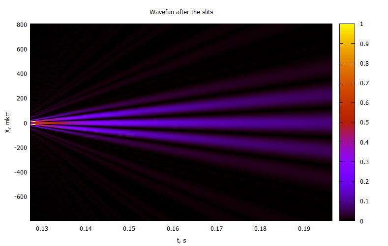
end

t₂(v, z) = sqrt( 2*(l1+l2-z)/g + (v/g)^2 ) - v/g
tf2 = t₂(v₀[3], 0) # s #    
X2 = range(-800, stop = 800, length = 200)*1e-6
Z2 = range(l1, stop = l2, length = 100)
Cron2 = range(tf1, stop = tf2, length = 100)

@time P2 = [ ρₓ(x, t) for t in Cron2, x in X2 ];

P2 /= maximum(P2[4:end,:]);
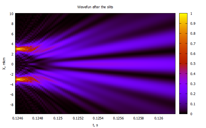
@gp "set title 'Wavefun after the slits'" xlab="t, s" ylab="X, mkm"
@gp :- Cron2[4:end] 1000000X2 P2[4:end,:] "w image notit"

2 :

\vec{v} = \frac{\nabla S}{m}

$\vec v = \frac{\nabla S}{m}$

. . , ,

\begin{aligned} \vec{v} (x, y, z, t) & = \frac{\nabla S}{m} + \frac{\nabla \log ρ \times \vec{s}}{m} \\ \vec{s} & = (0, 0, ℏ / 2) \\ \frac{\nabla \log ρ \times \vec{s}}{m} & = \frac{ℏ}{2 m ρ} (\frac{\partial ρ}{\partial y}, - \frac{\partial ρ}{\partial x}, 0) \end{aligned}

$\begin{aligned} \vec v(x, y, z, t)&=\frac{\nabla S}{m}+\frac{\nabla \log \rho \times \vec s}{m} \\ \vec s &= (0,0,\hbar/2)\\ \frac{\nabla \log \rho \times \vec s}{m} &= \frac{\hbar}{2 m \rho}\left( \frac{\partial \rho}{\partial y}, -\frac{\partial \rho}{\partial x}, 0\right) \end{aligned}$

, ,

\begin{aligned} \frac{d x}{d t} & = v_{x} (x, t) = \frac{1}{m} \frac{\partial S}{\partial x} + \frac{ℏ}{2 m ρ} \frac{\partial ρ}{\partial y} = v_{0 x} + \frac{(x - v_{0 x} t) ℏ^{2} t}{4 m^{2} σ_{0}^{2} σ_{0}^{2} (t)} - \frac{ℏ (y - v_{0 y} t)}{2 m σ_{0}^{2} (t)} \\ \frac{d y}{d t} & = v_{y} (x, t) = \frac{1}{m} \frac{\partial S}{\partial y} - \frac{ℏ}{2 m ρ} \frac{\partial ρ}{\partial x} = v_{0 y} - \frac{(y - v_{0 y} t) ℏ^{2} t}{4 m^{2} σ_{0}^{2} σ_{0}^{2} (t)} + \frac{ℏ (x - v_{0 x} t)}{2 m σ_{0}^{2} (t)} \\ \frac{d z}{d t} & = v_{z} (z, t) = \frac{1}{m} \frac{\partial S}{\partial z} = v_{0 z} + g t + \frac{(z - v_{0 z} t - g t^{2} / 2) ℏ^{2} t}{4 m^{2} σ_{z}^{2} σ_{z}^{2} (t)} \end{aligned}

$\begin{aligned} \frac{d x}{d t} &=v_{x}(x, t)=\frac{1}{m} \frac{\partial S}{\partial x}+\frac{\hbar}{2 m \rho} \frac{\partial \rho}{\partial y}=v_{0 x}+\frac{\left(x-v_{0 x} t\right) \hbar^{2} t}{4 m^{2} \sigma_{0}^{2} \sigma_{0}^{2}(t)}-\frac{\hbar\left(y-v_{0 y} t\right)}{2 m \sigma_{0}^{2}(t)} \\ \frac{d y}{d t} &=v_{y}(x, t)=\frac{1}{m} \frac{\partial S}{\partial y}-\frac{\hbar}{2 m \rho} \frac{\partial \rho}{\partial x}=v_{0 y}-\frac{\left(y-v_{0 y} t\right) \hbar^{2} t}{4 m^{2} \sigma_{0}^{2} \sigma_{0}^{2}(t)}+\frac{\hbar\left(x-v_{0 x} t\right)}{2 m \sigma_{0}^{2}(t)} \\ \frac{d z}{d t} &= v_{z}(z, t)=\frac{1}{m} \frac{\partial S}{\partial z}=v_{0 z}+g t+\frac{\left(z-v_{0 z} t-g t^{2} / 2\right) \hbar^{2} t}{4 m^{2} \sigma_{z}^{2} \sigma_{z}^{2}(t)} \end{aligned}$

\begin{aligned} x (t) & = v_{0 x} t + \sqrt{x_{0}^{2} + y_{0}^{2}} \frac{σ_{0} (t)}{σ_{0}} \cos φ (t) \\ y (t) & = v_{0 y} t + \sqrt{x_{0}^{2} + y_{0}^{2}} \frac{σ_{0} (t)}{σ_{0}} \sin φ (t) \\ z (t) & = v_{0 z} t + \frac{1}{2} g t^{2} + z_{0} \frac{σ_{z} (t)}{σ_{z}} \end{aligned}

$\begin{aligned} x(t) &=v_{0 x} t+\sqrt{x_{0}^{2}+y_{0}^{2}} \frac{\sigma_{0}(t)}{\sigma_{0}} \cos \varphi(t) \\ y(t) &=v_{0 y} t+\sqrt{x_{0}^{2}+y_{0}^{2}} \frac{\sigma_{0}(t)}{\sigma_{0}} \sin \varphi(t)\\ z(t) &= v_{0 z} t+\frac{1}{2} g t^{2}+z_{0} \frac{\sigma_{z}(t)}{\sigma_{z}} \end{aligned}$

\begin{aligned} σ_{0}^{2} (t) & = σ_{0}^{2} + {(\frac{ℏ t}{2 m σ_{0}})}^{2} \\ φ (t) & = φ_{0} + \arctan (- \frac{ℏ t}{2 m σ_{0}^{2}}) \\ \cos (φ_{0}) & = \frac{x_{0}}{\sqrt{x_{0}^{2} + y_{0}^{2}}} \\ \sin (φ_{0}) & = \frac{y_{0}}{\sqrt{x_{0}^{2} + y_{0}^{2}}} \\ \sin (\arctan x) & = \frac{x}{\sqrt{1 + x^{2}}} \\ \cos (\arctan x) & = \frac{1}{\sqrt{1 + x^{2}}} \\ \cos (a + b) & = \cos a \cos b - \sin a \sin b \\ \sin (a + b) & = \sin a \cos b + \cos a \sin b \end{aligned}

$\begin{aligned} \sigma_{0}^{2}(t) &= \sigma_{0}^{2}+\left(\frac{\hbar t}{2 m \sigma_{0}}\right)^{2} \\ \varphi(t) &= \varphi_{0}+\arctan \left(-\frac{\hbar t}{2 m \sigma_{0}^{2}}\right) \\ \cos \left(\varphi_{0}\right) &= \frac{x_{0}}{\sqrt{x_{0}^{2}+y_{0}^{2}}} \\ \sin \left(\varphi_{0}\right) &= \frac{y_{0}}{\sqrt{x_{0}^{2}+y_{0}^{2}} } \\ \sin(\arctan x) &= \frac{x}{\sqrt{1+x^2}} \\ \cos(\arctan x) &= \frac{1}{\sqrt{1+x^2}} \\ \cos(a+b) &= \cos a\cos b - \sin a\sin b \\ \sin(a+b) &= \sin a\cos b + \cos a\sin b \end{aligned}$

function xbs(t, xo, yo, vo)

    cosϕ = xo / sqrt( xo^2 + yo^2 )
    sinϕ = yo / sqrt( xo^2 + yo^2 )
    atnx = -ħ*t / (2m*σ₀^2)
    sinatnx = atnx / sqrt( atnx^2 + 1)
    cosatnx =    1 / sqrt( atnx^2 + 1)
    cosϕt = cosϕ * cosatnx - sinϕ * sinatnx
    #sinϕt = sinϕ*cosatnx + cosϕ*sinatnx

    σ₀t = sqrt( σ₀^2 + ( ħ*t / (2*m*σ₀) )^2 )

    vo*t + sqrt(xo^2 + yo^2) * σ₀t/σ₀ * cosϕt
end

@gp "set title 'Trajectories before slits'" xlab="t, s" ylab="X, mkm" # "set yrange [-10:10]"

@time for i in 1:80

    x0 = randn()*σ₀
    y0 = randn()*σ₀
    v0 = randn()*σv*1e-4

    prtclᵢ = [ xbs(t,x0,y0,v0) for t in Cron1 ]

    @gp :- Cron1 1000000prtclᵢ "with lines notit lw 2 lc rgb 'black'"
    # slits -4-> -2, 2->4 mkm
end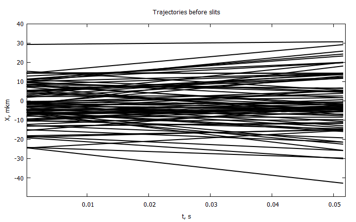

, , , , , . . . , .

Y , , . X . .

" " ,

v_{x} (x, t) = \frac{1}{t - t_{1}} [x + \frac{- 1}{2 (α^{2} + β_{t}^{2})} (β_{t} I m (\frac{C (x, t)}{H (x, t)}) + α Re (\frac{C (x, t)}{H (x, t)}) - β_{t} γ_{x, t})]

$v_{x}(x, t)=\frac{1}{t-t_{1}}\left[x+\frac{-1}{2\left(\alpha^{2}+\beta_{t}^{2}\right)}\left(\beta_{t} I m\left(\frac{C(x, t)}{H(x, t)}\right)+\alpha \operatorname{Re}\left(\frac{C(x, t)}{H(x, t)}\right)-\beta_{t} \gamma_{x, t}\right)\right]$

18+

\begin{aligned} H (x, t) & = \int_{X_{A} - b}^{X_{A} + b} f (x, u, t) d u + \int_{X_{B} - b}^{X_{B} + b} f (x, u, t) d u \\ C (x, t) & = [f (x, u, t)]_{u = X_{A} - b}^{u = X_{A} + b} + [f (x, u, t)]_{u = X_{B} - b}^{u = X_{B} + b} \\ f (x, u, t) & = \exp [(α + i β_{t}) u^{2} + i γ_{x, t} u] \\ α & = - \frac{1}{4 σ_{0}^{2} (1 + {(\frac{ℏ t_{1}}{2 m σ_{0}^{2}})}^{2})} \\ β_{t} & = \frac{m}{2 ℏ} (\frac{1}{t - t_{1}} + \frac{1}{t_{1} (1 + {(\frac{2 m σ_{0}^{2}}{ℏ t_{1}})}^{2})}) \\ γ_{x, t} & = - \frac{m x}{ℏ (t - t_{1})} \end{aligned}

$\begin{aligned} H(x, t) &= \int_{X_{A}-b}^{X_{A}+b} f(x, u, t) d u+\int_{X_{B}-b}^{X_{B}+b} f(x, u, t) d u \\ C(x, t) &= [f(x, u, t)]_{u=X_{A}-b}^{u=X_{A}+b}+[f(x, u, t)]_{u=X_{B}-b}^{u=X_{B}+b} \\ f(x, u, t) &= \exp \left[\left(\alpha+i \beta_{t}\right) u^{2}+i \gamma_{x, t} u\right]\\ \alpha &= -\frac{1}{4 \sigma_{0}^{2}\left(1+\left(\frac{\hbar t_{1}}{2 m \sigma_{0}^{2}}\right)^{2}\right)} \\ \beta_{t} &= \frac{m}{2 \hbar}\left(\frac{1}{t-t_{1}}+\frac{1}{t_{1}\left(1+\left(\frac{2 m \sigma_{0}^{2}}{\hbar t_{1}}\right)^{2}\right)}\right) \\ \gamma_{x, t} &= -\frac{m x}{\hbar\left(t-t_{1}\right)} \end{aligned}$

function Uₓ(t, x)

    γ = -m*x / ( ħ*(t-tf1) )
    β = m/(2ħ) * ( 1/(t-tf1) + 1 / ( tf1*( 1 + (2m*σ₀^2 / (ħ*tf1) )^2 ) ) )
    α = -( 4σ₀^2 * ( 1 + ( ħ*tf1 / (2m*σ₀^2) )^2 ) )^-1

    f(x, u, t) = exp( ( α + im*β )*u^2 + im*γ*u )

    C = f(x, a2, t) - f(x, a1, t) + f(x, b2, t) - f(x, b1, t)
    H = trapez( u-> f(x, u, t) , a1, a2, 400) + trapez( u-> f(x, u, t) , b1, b2, 400)

    return 1/(t-tf1) * ( x - 0.5/(α^2 + β^2) * ( β*imag(C/H) + α*real(C/H) - β*γ ) )
end

init() = bitrand()[1] ? rand()*(b2 - b1) + b1 : rand()*(a2 - a1) + a1
myrng(a, b, N) = collect( range(a, stop = b, length = N ÷ 2) )

n = 1
xx = 0
ξ = 1e-5
while xx < Cron2[end]-Cron2[1]
    n+=1
    xx += (ξ*n)^2 
end
n

steps = [ (ξ*i)^2 for i in 1:n1 ]
Cronadapt = accumulate(+, steps, init = Cron2[1] )

function modelsolver(Np = 10, Nt = 100)

    #xo = [ init() for i = 1:Np ] # 
    xo = vcat( myrng(a2, a1, Np), myrng(b1, b2, Np) ) # 

    xpath = zeros(Nt, Np)
    xpath[1,:] = xo

    for i in 2:Nt, j in 1:Np
        xpath[i,j] = rk4(Uₓ, Cronadapt[i], xpath[i-1,j], steps[i] )
    end

    xpath
end

@time paths = modelsolver(20, n);

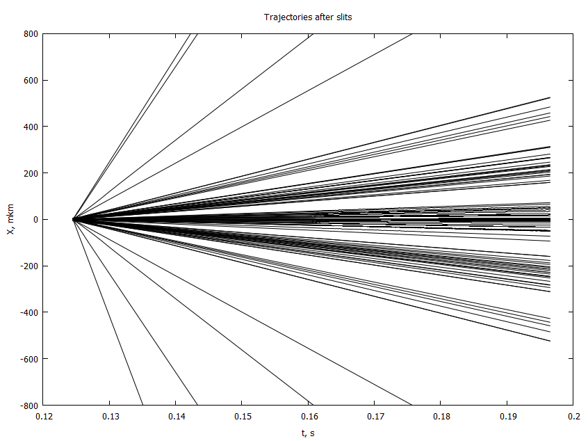
@gp "set title 'Trajectories after the slits'" xlab="t, s" ylab="X, mkm" "set yrange [-800:800]"
for i in 1:size(paths, 2)
    @gp :- Cronadapt 1e6paths[:,i] "with lines notit lw 1 lc rgb 'black'"
end

- 4 , . 2

, : , , .

. , ,

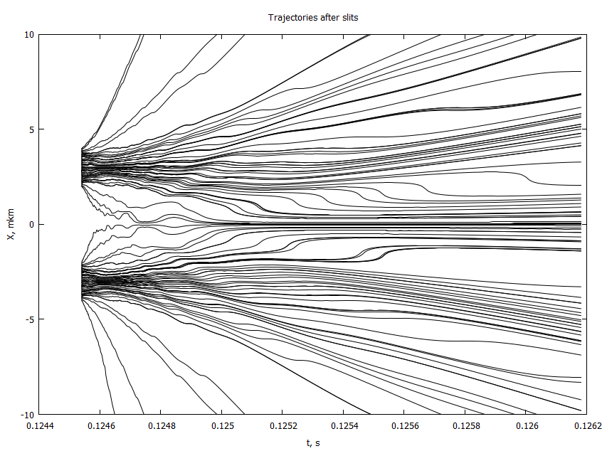
function yas(t, xo, yo, vo)

    cosϕ = xo / sqrt( xo^2 + yo^2 )
    sinϕ = yo / sqrt( xo^2 + yo^2 )
    atnx = -ħ*t / (2m*σ₀^2)
    sinatnx = atnx / sqrt( atnx^2 + 1)
    cosatnx =    1 / sqrt( atnx^2 + 1)
    #cosϕt = cosϕ * cosatnx - sinϕ * sinatnx
    sinϕt = sinϕ*cosatnx + cosϕ*sinatnx

    σ₀t = sqrt( σ₀^2 + ( ħ*t / (2*m*σ₀) )^2 )

    vo*t + sqrt(xo^2 + yo^2) * σ₀t/σ₀ * sinϕt
end

function modelsolver2(Np = 10)

    Nt = length(Cronadapt)
    xo = [ init() for i = 1:Np ]
    #xo = vcat( myrng(a2, a1, Np), myrng(b1, b2, Np) )

    xcoord = copy(xo)
    ycoord = zeros(Np)

    for i in 2:Nt, j in 1:Np
        xcoord[j] = rk4(Uₓ, Cronadapt[i], xcoord[j], steps[i] )
    end

    for (i, x) in enumerate(xo)

        y0 = randn()*yh
        v0 = 0 #randn()*σv*1e-4

        ycoord[i] = yas(Cronadapt[end], x, y0, v0)
    end

    xcoord, ycoord
end

@time X, Y = modelsolver2(100);

@gp "set title 'Impacts on the screen'" xlab="X, mm" ylab="Y, mm"# "set xrange [-1:1]"
@gp :- 1000X 1000Y "with points notit pt 7 ps 0.5 lc rgb 'black'"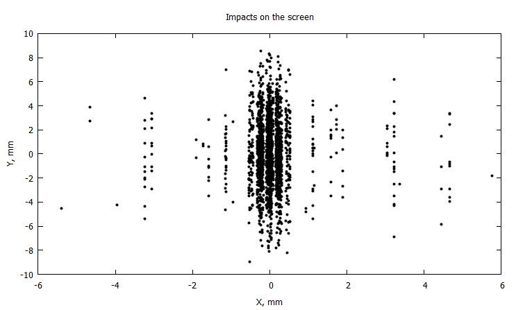

, , . , ,

, , , , , — , .

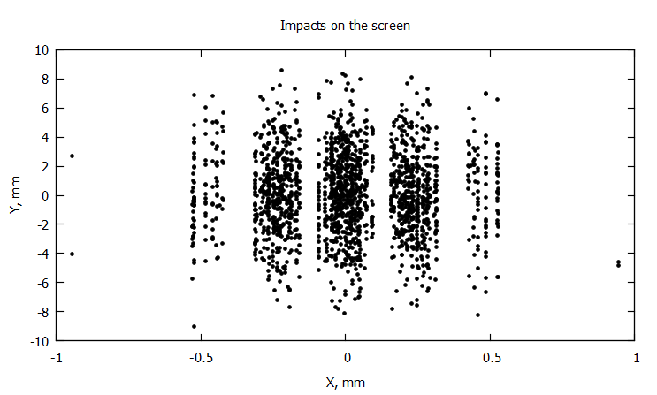
わいせつなアプリケーション

More articles: