ブラウザでTensorFlow.jsを使用する利点
- インタラクティブ性-ブラウザには、進行中のプロセス(グラフィック、アニメーションなど)を視覚化するための多くのツールがあります。
- センサー-ブラウザーはデバイスのセンサー(カメラ、GPS、加速度計など)に直接アクセスできます。
- ユーザーデータのセキュリティ-処理されたデータをサーバーに送信する必要はありません。
- Pythonで作成されたモデルとの互換性。
パフォーマンス
主な問題の1つはパフォーマンスです。
実際、機械学習はマトリックスのようなデータ(テンサー)を使用してさまざまな種類の数学演算を実行しているため、ブラウザーでのこの種の計算用のライブラリーはWebGLを使用します。これにより、純粋なJSで同じ操作を実行した場合、パフォーマンスが大幅に向上します。当然、何らかの理由でWebGLがブラウザでサポートされていない場合、ライブラリにはフォールバックがあります(この記事の執筆時点では、caniuseはユーザーの97.94%がWebGLをサポートしていることを示しています)。
パフォーマンスを向上させるために、Node.jsはTensorFlowでネイティブバインディングを使用します。ここでは、CPU、GPU、TPU(テンソルプロセッシングユニット)がアクセラレータとして機能します。
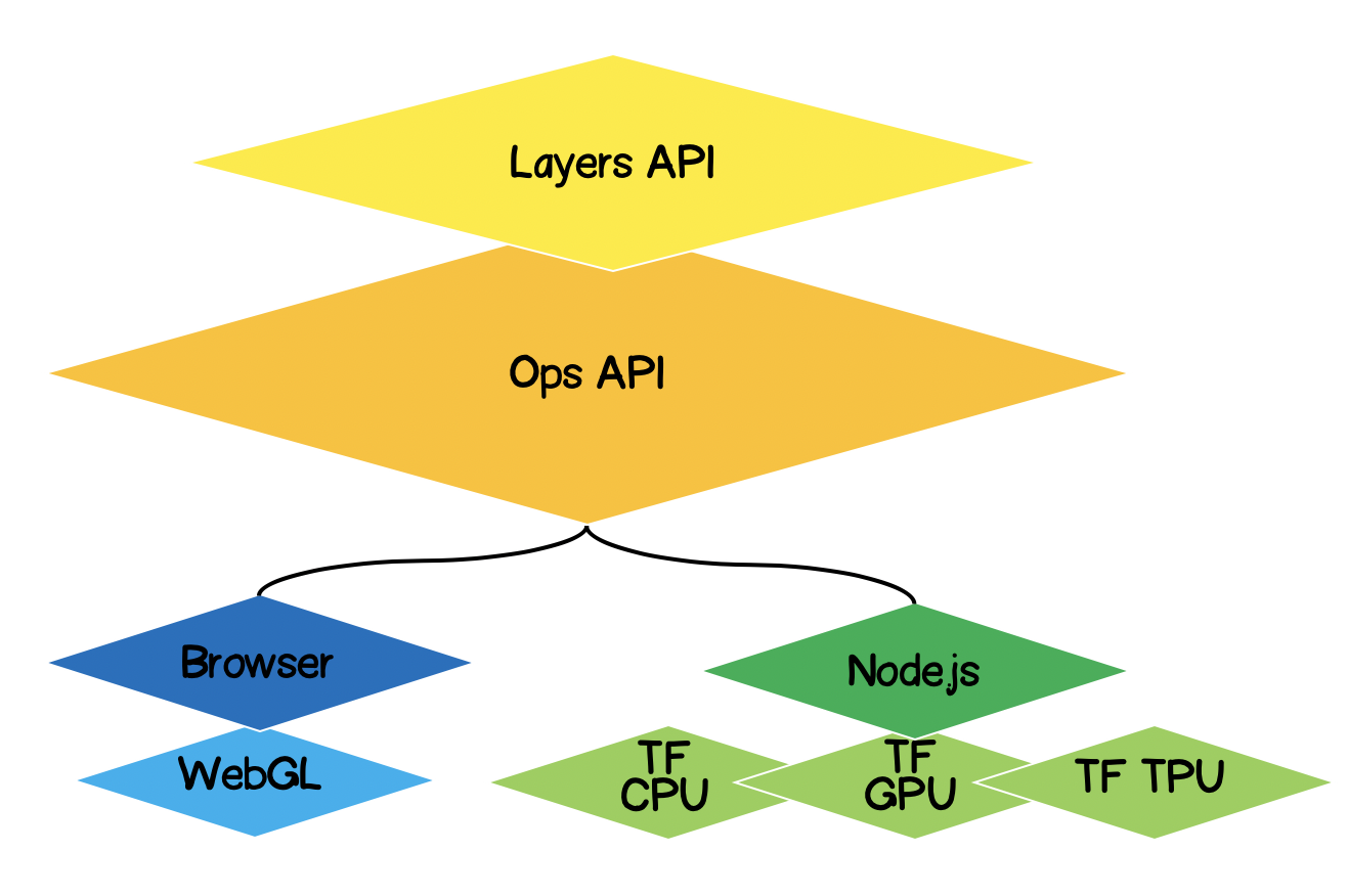
TensorFlow.jsアーキテクチャ
- 最下位層-この層は、テンサーで数学演算を実行する際の計算の並列化を担当します。
- オプスのAPI -テンソルでは、数学的な演算を実行するためのAPIを提供します。
- Layers API-さまざまなタイプのレイヤー(高密度、畳み込み)を使用して、ニューラルネットワークの複雑なモデルを作成できます。このレイヤーはKerasPython APIに似ており、事前にトレーニングされたKerasPythonベースのネットワークをロードする機能があります。
問題の定式化
与えられた一連の実験点について、近似線形関数の方程式を見つける必要があります。言い換えれば、実験点に最も近い線形曲線を見つける必要があります。

ソリューションの形式化
機械学習の中核はモデルになります。この場合、これは線形関数の方程式です。
条件に基づいて、一連の実験ポイントもあります。
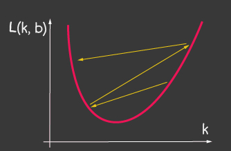
それを仮定します -トレーニングの第ステップでは、線形方程式の次の係数が計算されました ..。次に、選択した係数の正確さを数学的に表現する必要があります。これを行うには、たとえば標準偏差によって決定できるエラー(損失)を計算する必要があります。Tensorflow.jsは、一般的に使用される損失関数のセットを提供します:tf.metrics.meanAbsoluteError、tf.metrics.meanSquaredErrorなど。
近似の目的は、エラー関数を最小化することです ..。これには勾配降下法を使用しましょう。これは必要である:
- — -, ;
- — -. , :
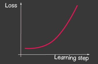
— (learning rate) . . learning rate ( 2), — , 1.
|


|
|---|---|
| 1: (learning-rate) | 2: (learning-rate) |
Tensorflow.js
たとえば、損失関数の値(標準偏差)の計算は次のようになります。
function loss(ysPredicted, ysReal) {
    const squaredSum = ysPredicted.reduce(
        (sum, yPredicted, i) => sum + (yPredicted - ysReal[i]) ** 2,
        0);
    return squaredSum / ysPredicted.length;
}
ただし、入力データの量は多くなる可能性があります。モデルのトレーニング中に、各反復での損失関数の値を計算するだけでなく、より深刻な操作(勾配の計算)も実行する必要があります。したがって、WebGLを使用して計算を最適化するtensorflowを使用することは理にかなっています。さらに、コードははるかに表現力豊かになります。比較してください。
    function loss(ysPredicted, ysReal) => {
        const ysPredictedTensor = tf.tensor(ysPredicted);
        const ysRealTensor = tf.tensor(ysReal);
        const loss = ysPredictedTensor.sub(ysRealTensor).square().mean();
        return loss.dataSync()[0];
    };
TensorFlow.jsを使用したソリューション
幸いなことに、特定のエラー関数(損失)に対してオプティマイザーを作成する必要はありません。部分導関数を計算するための数値メソッドを開発する必要はありません。すでに逆伝播アルゴリズムを実装しています。次の手順に従う必要があります。
- モデルを設定します(この場合は線形関数)。
- エラー関数を記述します(この場合、これは標準偏差です)
- 実装されているオプティマイザの1つを選択します(独自の実装でライブラリを拡張することは可能です)
テンソルとは
絶対に誰もが数学のテンサーに出くわしました-これらはスカラー、ベクトル、2D-マトリックス、3D-マトリックスです。テンソルは、上記のすべての一般化された概念です。これは、同種タイプ(tensorflowはint32、float32、bool、complex64、stringをサポート)のデータを含み、特定の形状(軸の数(ランク)と各軸の要素の数)を持つデータコンテナーです。以下では、3Dマトリックスまでのテンサーについて検討しますが、これは一般化であるため、テンサーは5D、6D、... NDなどの軸をいくつでも持つことができます。
TensorFlowには、テンソル生成用に次のAPIがあります。
tf.tensor (values, shape?, dtype?)ここで、shapeはテンソルの形状であり、配列によって与えられます。ここで、要素の数は軸の数であり、配列の各値によって、各軸に沿った要素の数が決まります。たとえば、4x2マトリックス(4行2列)を定義する場合、フォームは[4、2]の形式になります。
| 視覚化 | 説明 |
|---|---|

|
スカラー
ランク:0 フォーム:[] JS構造: TensorFlow API: |

|
ベクトル
ランク:1 形状:[4] JS構造: TensorFlow API: |
 |
マトリックス
ランク:2 形状:[4,2] JS構造: TensorFlow API: |
 |
マトリックス
ランク:3 形状:[4,2,3] JS構造: TensorFlow API: |
TensorFlow.jsによる線形近似
最初に、コードを拡張可能にすることについて説明します。線形近似を、あらゆる種類の関数によって実験点の近似に変換できます。クラス階層は次のようになります。

子クラスで定義される抽象メソッドを除いて、抽象クラスのメソッドの実装を開始しましょう。ここでは、何らかの理由でメソッドが子クラスで定義されていない場合にのみ、スタブにエラーを残します。
import * as tf from '@tensorflow/tfjs';

export default class AbstractRegressionModel {
    constructor(
        width,
        height,
        optimizerFunction = tf.train.sgd,
        maxEpochPerTrainSession = 100,
        learningRate = 0.1,
        expectedLoss = 0.001
    ) {
        this.width = width;
        this.height = height;
        this.optimizerFunction = optimizerFunction;
        this.expectedLoss = expectedLoss;
        this.learningRate = learningRate;
        this.maxEpochPerTrainSession = maxEpochPerTrainSession;

        this.initModelVariables();

        this.trainSession = 0;
        this.epochNumber = 0;
        this.history = [];
    }
}したがって、モデルのコンストラクターで、幅と高さを定義しました。これらは、実験ポイントを配置する平面の実際の幅と高さです。これは、入力データを正規化するために必要です。それら。私たちが持っている場合、次に正規化後、次のようになります。
optimizerFunction-ライブラリで利用可能な他のオプティマイザを試すことができるように、オプティマイザのタスクを柔軟にします。デフォルトでは、確率的勾配降下メソッドtf.train.sgdを設定しています。また、トレーニング中にlearningRateを微調整でき、学習プロセスが大幅に改善される他の利用可能なオプティマイザーで遊ぶことをお勧めします。たとえば、次のオプティマイザーを試してください:tf.train.momentum、tf.train.adam。
学習プロセスが無限ではないように、maxEpochPerTrainSesionとexpectedLossの2つのパラメーターを定義しました。-このようにして、トレーニングの最大反復回数に達したとき、またはエラー関数の値が予想されるエラーよりも低くなったときに、トレーニングプロセスを停止します(以下のtrainメソッドですべてを考慮します)。
コンストラクターでは、initModelVariablesメソッドを呼び出しますが、合意されているように、後で子クラスでスタブして定義します。
initModelVariables() {
    throw Error('Model variables should be defined')
}
次に、トレインモデルのメインメソッドを実装しましょう。
/**
     * Train model until explicitly stop process via invocation of stop method
     * or loss achieve necessary accuracy, or train achieve max epoch value
     *
     * @param x - array of x coordinates
     * @param y - array of y coordinates
     * @param callback - optional, invoked after each training step
     */
    async train(x, y, callback) {
        const currentTrainSession = ++this.trainSession;
        this.lossVal = Number.POSITIVE_INFINITY;
        this.epochNumber = 0;
        this.history = [];

        // convert array into tensors
        const input = tf.tensor1d(this.xNormalization(x));
        const output = tf.tensor1d(this.yNormalization(y));

        while (
            currentTrainSession === this.trainSession
            && this.lossVal > this.expectedLoss
            && this.epochNumber <= this.maxEpochPerTrainSession
            ) {
            const optimizer = this.optimizerFunction(this.learningRate);
            optimizer.minimize(() => this.loss(this.f(input), output));
            this.history = [...this.history, {
                epoch: this.epochNumber,
                loss: this.lossVal
            }];
            callback && callback();
            this.epochNumber++;
            await tf.nextFrame();
        }
    }
trainSessionは基本的に、前のトレーニングセッションがまだ終了していないときに、外部APIがtrainメソッドを呼び出す場合の、トレーニングセッションの一意の識別子です。
コードから、1次元配列からtensor1dを作成していることがわかります。データは事前に正規化する必要がありますが、正規化の関数は次のとおりです。
xNormalization = xs => xs.map(x => x / this.width);
yNormalization = ys => ys.map(y => y / this.height);
yDenormalization = ys => ys.map(y => y * this.height);
ループでは、トレーニングステップごとに、モデルオプティマイザーを呼び出します。これに、損失関数を渡す必要があります。合意されたように、損失関数は標準偏差によって設定されます。次に、APItensorflow.jsを使用します。
    /**
     * Calculate loss function as mean-square deviation
     *
     * @param predictedValue - tensor1d - predicted values of calculated model
     * @param realValue - tensor1d - real value of experimental points
     */
    loss = (predictedValue, realValue) => {
        // L = sum ((x_pred_i - x_real_i)^2) / N
        const loss = predictedValue.sub(realValue).square().mean();
        this.lossVal = loss.dataSync()[0];
        return loss;
    };
学習プロセスは継続します
- 反復回数の制限には達しません
- 望ましいエラー精度が達成されない
- 新しいトレーニングプロセスは開始されていません
また、損失関数がどのように呼び出されるかに注意してください。予測値を取得するために(関数fを呼び出します)、実際には、回帰が実行される形式を設定し、合意されたように、抽象クラスにスタブを配置します。
  f(x) {
        throw Error('Model should be defined')
  }
トレーニングの各ステップで、履歴モデルのオブジェクトのプロパティに、各トレーニングエポックでのエラー変更のダイナミクスを保存します。
モデルのトレーニングプロセスの後、トレーニングされたモデルを使用して、入力を受け入れ、計算された出力を出力するメソッドが必要です。これを行うために、APIでpredictメソッドを定義しました。これは次のようになります。
/**
     * Predict value basing on trained model
     *  @param x - array of x coordinates
     *  @return Array({x: integer, y: integer}) - predicted values associated with input
     *
     * */
    predict(x) {
        const input = tf.tensor1d(this.xNormalization(x));
        const output = this.yDenormalization(this.f(input).arraySync());
        return output.map((y, i) => ({ x: x[i], y }));
    }
node.jsと同様に、arraySyncに 注意してください。arraySyncメソッドがある場合は、Promiseを返す非同期配列メソッドが確実にあります。先に述べたように、計算を高速化するためにテンサーはすべてWebGLに移行され、WebGLからJS変数にデータを移動するのに時間がかかるため、プロセスは非同期になるため、ここでPromiseが必要です。
抽象クラスが完成しました。コードの完全版は次の場所にあります。
AbstractRegressionModel.js
import * as tf from '@tensorflow/tfjs';

export default class AbstractRegressionModel {

    constructor(
        width,
        height,
        optimizerFunction = tf.train.sgd,
        maxEpochPerTrainSession = 100,
        learningRate = 0.1,
        expectedLoss = 0.001
    ) {
        this.width = width;
        this.height = height;
        this.optimizerFunction = optimizerFunction;
        this.expectedLoss = expectedLoss;
        this.learningRate = learningRate;
        this.maxEpochPerTrainSession = maxEpochPerTrainSession;

        this.initModelVariables();

        this.trainSession = 0;
        this.epochNumber = 0;
        this.history = [];
    }

    initModelVariables() {
        throw Error('Model variables should be defined')
    }

    f() {
        throw Error('Model should be defined')
    }

    xNormalization = xs => xs.map(x => x / this.width);
    yNormalization = ys => ys.map(y => y / this.height);
    yDenormalization = ys => ys.map(y => y * this.height);

    /**
     * Calculate loss function as mean-squared deviation
     *
     * @param predictedValue - tensor1d - predicted values of calculated model
     * @param realValue - tensor1d - real value of experimental points
     */
    loss = (predictedValue, realValue) => {
        const loss = predictedValue.sub(realValue).square().mean();
        this.lossVal = loss.dataSync()[0];
        return loss;
    };

    /**
     * Train model until explicitly stop process via invocation of stop method
     * or loss achieve necessary accuracy, or train achieve max epoch value
     *
     * @param x - array of x coordinates
     * @param y - array of y coordinates
     * @param callback - optional, invoked after each training step
     */
    async train(x, y, callback) {
        const currentTrainSession = ++this.trainSession;
        this.lossVal = Number.POSITIVE_INFINITY;
        this.epochNumber = 0;
        this.history = [];

        // convert data into tensors
        const input = tf.tensor1d(this.xNormalization(x));
        const output = tf.tensor1d(this.yNormalization(y));

        while (
            currentTrainSession === this.trainSession
            && this.lossVal > this.expectedLoss
            && this.epochNumber <= this.maxEpochPerTrainSession
            ) {
            const optimizer = this.optimizerFunction(this.learningRate);
            optimizer.minimize(() => this.loss(this.f(input), output));
            this.history = [...this.history, {
                epoch: this.epochNumber,
                loss: this.lossVal
            }];
            callback && callback();
            this.epochNumber++;
            await tf.nextFrame();
        }
    }

    stop() {
        this.trainSession++;
    }

    /**
     * Predict value basing on trained model
     *  @param x - array of x coordinates
     *  @return Array({x: integer, y: integer}) - predicted values associated with input
     *
     * */
    predict(x) {
        const input = tf.tensor1d(this.xNormalization(x));
        const output = this.yDenormalization(this.f(input).arraySync());
        return output.map((y, i) => ({ x: x[i], y }));
    }
}
線形回帰の場合、抽象クラスから継承する新しいクラスを定義します。ここでは、2つのメソッドinitModelVariablesとfを定義するだけで済みます。
線形近似に取り組んでいるため、2つの変数k、bを指定する必要があります。これらはスカラーテンサーになります。オプティマイザの場合、それらが調整可能(変数)であることを示し、初期値として任意の数値を割り当てる必要があります。
initModelVariables() {
   this.k = tf.scalar(Math.random()).variable();
   this.b = tf.scalar(Math.random()).variable();
}
ここ で変数のAPIを検討してください:
tf.variable (initialValue, trainable?, name?, dtype?)trainable の2番目の引数であるブール変数に注意してください。デフォルトではtrueです。オプティマイザによって使用され、損失関数を最小化するときにこの変数を構成する必要があるかどうかを通知します。これは、Keras Pythonからダウンロードした事前トレーニング済みモデルに基づいて新しいモデルを構築する場合に役立ちます。また、このモデルの一部のレイヤーを再トレーニングする必要はないと確信しています。
次に、tensorflow APIを使用して近似関数の方程式を定義する必要があります。コードを見ると、その使用方法を直感的に理解できます。
f(x) {
   // y = kx + b
   return  x.mul(this.k).add(this.b);
}
たとえば、この方法で2次近似を指定できます。
initModelVariables() {
   this.a = tf.scalar(Math.random()).variable();
   this.b = tf.scalar(Math.random()).variable();
   this.c = tf.scalar(Math.random()).variable();
}

f(x) {
    // y = ax^2 + bx + c
    return this.a.mul(x.square()).add(this.b.mul(x)).add(this.c);
}
ここでは、線形および2次回帰のモデルを確認できます。
LinearRegressionModel.js
import * as tf from '@tensorflow/tfjs';
import AbstractRegressionModel from "./AbstractRegressionModel";

export default class LinearRegressionModel extends AbstractRegressionModel {
    initModelVariables() {
        this.k = tf.scalar(Math.random()).variable();
        this.b = tf.scalar(Math.random()).variable();
    }

    f = x => x.mul(this.k).add(this.b);
}
QuadraticRegressionModel.js
import * as tf from '@tensorflow/tfjs';
import AbstractRegressionModel from "./AbstractRegressionModel";

export default class QuadraticRegressionModel extends AbstractRegressionModel {
    initModelVariables() {
        this.a = tf.scalar(Math.random()).variable();
        this.b = tf.scalar(Math.random()).variable();
        this.c = tf.scalar(Math.random()).variable();
    }

    f = x => this.a.mul(x.square()).add(this.b.mul(x)).add(this.c);
}
以下は、記述された線形回帰モデルを使用し、ユーザーのUXを作成するReactで記述されたコードです。
Regression.js
import React, { useState, useEffect } from 'react';

import Canvas from './components/Canvas';
import LossPlot from './components/LossPlot_v3';
import LinearRegressionModel from './model/LinearRegressionModel';

import './RegressionModel.scss';

const WIDTH = 400;
const HEIGHT = 400;
const LINE_POINT_STEP = 5;

const predictedInput = Array.from({ length: WIDTH / LINE_POINT_STEP + 1 })
    .map((v, i) => i * LINE_POINT_STEP);

const model = new LinearRegressionModel(WIDTH, HEIGHT);

export default () => {
    const [points, changePoints] = useState([]);
    const [curvePoints, changeCurvePoints] = useState([]);
    const [lossHistory, changeLossHistory] = useState([]);

    useEffect(() => {
        if (points.length > 0) {
            const input = points.map(({ x }) => x);
            const output = points.map(({ y }) => y);

            model.train(input, output, () => {
                changeCurvePoints(() => model.predict(predictedInput));
                changeLossHistory(() => model.history);
            });
        }
    }, [points]);

    return (
        <div className="regression-low-level">
            <div className="regression-low-level__top">
                <div className="regression-low-level__workarea">
                    <div className="regression-low-level__canvas">
                        <Canvas
                            width={WIDTH}
                            height={HEIGHT}
                            points={points}
                            curvePoints={curvePoints}
                            changePoints={changePoints}
                        />
                    </div>
                    <div className="regression-low-level__toolbar">
                        <button
                            className="btn btn-red"
                            onClick={() => model.stop()}>Stop
                        </button>
                        <button
                            className="btn btn-yellow"
                            onClick={() => {
                                model.stop();
                                changePoints(() => []);
                                changeCurvePoints(() => []);
                            }}>Clear
                        </button>
                    </div>
                </div>
                <div className="regression-low-level__loss">
                    <LossPlot
                              loss={lossHistory}/>
                </div>

            </div>
        </div>
    )
}
結果:
次のタスクを実行することを強くお勧めします。
- 対数関数による関数近似を実装する
- tf.train.sgdオプティマイザーの場合は、learningRateで遊んで、学習プロセスの変化を確認してみてください。図2に示す画像を取得するには、learningRateを非常に大きく設定してみてください。
- オプティマイザをtf.train.adamに設定します。学習プロセスは改善されましたか?学習プロセスがモデルコンストラクターのlearningRate値の変更に依存しているかどうか。