
この記事では、ローン申請の履歴データを使用して、申請者がローンを返済できるかどうかを予測する(借り手のデフォルトのリスクを判断する)ことを目的とした、ホームクレジットデフォルトリスクマシンラーニングコンペティションについて説明し ます。顧客がローンを返済するかトラブルに遭遇するかを予測することは重要なビジネス上の課題であり、Home CreditはKaggleプラットフォームで競争を行って、コミュニティがこの課題を支援するために開発できる機械学習モデルを確認しています。
これは、標準の監視付き分類タスクです。
監視付き学習:正解はトレーニングデータに含まれています。目標は、利用可能な手がかりに基づいてこれらの応答を予測するようにモデルをトレーニングすることです。
: , – 0 ( ) 1 ( ).
Home Credit, () , . 7 :
applicationtrain / applicationtest: Home Credit. , SKIDCURR . TARGET :
0, ;
1, .
bureau: . , .
bureaubalance: . . , .
previousapplication: Home Credit , . , SKIDPREV.
POSCASHBALANCE: , Home Credit. , .
creditcardbalance: , Home Credit. . .
installments_payment: Home Credit, .
, :

, ( HomeCredit_columns_description.csv) .
(application_train / application_test), . , . , ! - , .
: ROC AUC
( ), , . , (ROC AUC, AUROC).
ROC AUC , , .
(ROC) , , , , :
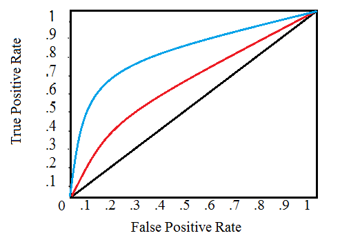
, , . 0 1 . , , . , , , , , , ( ).
(AUC) . ROC ( ). 0 1, . , , ROC AUC = 0,5.
ROC AUC, 0 1, 0 1. , , , ( , ) — . , , 99,9999%, , , . , ( ), , ROC AUC F1, . ROC AUC , ROC AUC .
, , . , , . .
: numpy pandas , sklearn preprocessing , matplotlib ¨C11C¨C12C¨C13C . .
import os
import numpy as np
import pandas as pd
pd.set_option('display.max_columns', None)
from sklearn.preprocessing import LabelEncoder
import matplotlib.pyplot as plt
import seaborn as sns
#
import warnings
warnings.filterwarnings('ignore')
, , . 9 : ( ), ( ), 6 , .
#
print(os.listdir("../input/"))
‘POSCASHbalance.csv’, ‘bureaubalance.csv’, ‘applicationtrain.csv’, ‘previousapplication.csv’, ‘installmentspayments.csv’, ‘creditcardbalance.csv’, ‘samplesubmission.csv’, ‘applicationtest.csv’, ‘bureau.csv’]
#
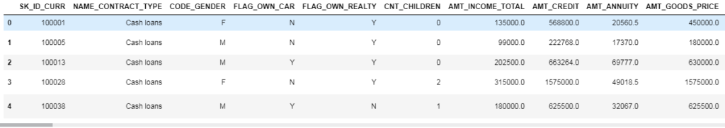
app_train = pd.read_csv('../input/application_train.csv')
print('Training data shape: ', app_train.shape)
app_train.head()
Training data shape: (307511, 122)

307511 , 120 , , .
#
app_test = pd.read_csv('../input/application_test.csv')
print('Testing data shape: ', app_test.shape)
app_test.head()
Testing data shape: (48744, 121)
, TARGET.
(EXPLORATORY DATA ANALYSIS – EDA)
(EDA) — , , , , . EDA — , . , , . , , , , .
— , : 0, , 1, . , .
app_train['TARGET'].value_counts()

app_train['TARGET'].astype(int).plot.hist();
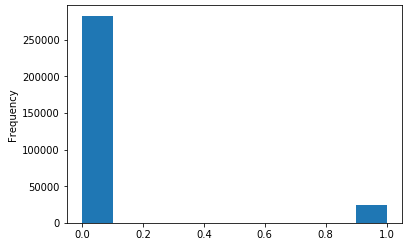
.
#
def missing_values_table(df):
#
mis_val = df.isnull().sum()
#
mis_val_percent = 100 * df.isnull().sum() / len(df)
#
mis_val_table = pd.concat([mis_val, mis_val_percent], axis=1)
#
mis_val_table_ren_columns = mis_val_table.rename(
columns = {0 : 'Missing Values', 1 : '% of Total Values'})
#
mis_val_table_ren_columns = mis_val_table_ren_columns[
mis_val_table_ren_columns.iloc[:,1] != 0].sort_values(
'% of Total Values', ascending=False).round(1)
#
print("Your selected dataframe has " + str(df.shape[1]) + " columns.\n"
"There are " + str(mis_val_table_ren_columns.shape[0]) +
" columns that have missing values.")
return mis_val_table_ren_columns
#
missing_values = missing_values_table(app_train)
missing_values.head(10)
Your selected dataframe has 122 columns.
There are 67 columns that have missing values.

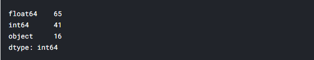
. int64 float64 — ( ). object .
#
app_train.dtypes.value_counts()
object().
#
app_train.select_dtypes('object').apply(pd.Series.nunique, axis = 0)

, . .
, . , ( , LightGBM). , () , . :
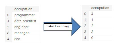
(Label encoding): . . :
(One-hot encoding): . 1 0 .

, . , , - . 4, — 1, , . . , , (, = 4 = 1) , , . (, / ), , .
, , . – Kaggle-master Will Koehrsen, , , . . , ( ) - . , PCA , ( , ).
Label Encoding 2 One-Hot Encoding 2 . , , , , . - .
Label Encoding One-Hot Encoding
: (dtype == object) , – .
LabelEncoder Scikit-Learn, – pandas get_dummies(df).
# label encoder
le = LabelEncoder()
le_count = 0
#
for col in app_train:
if app_train[col].dtype == 'object':
# 2
if len(list(app_train[col].unique())) <= 2:
# LabelEncoder
le.fit(app_train[col])
#
app_train[col] = le.transform(app_train[col])
app_test[col] = le.transform(app_test[col])
# , LabelEncoder
le_count += 1
print('%d columns were label encoded.' % le_count)
3 columns were label encoded.
# one-hot encoding
app_train = pd.get_dummies(app_train)
app_test = pd.get_dummies(app_test)
print('Training Features shape: ', app_train.shape)
print('Testing Features shape: ', app_test.shape)
raining Features shape: (307511, 243)
Testing Features shape: (48744, 239).
(). , , . . ( , ). , axis = 1, , !
train_labels = app_train['TARGET']
# , ,
app_train, app_test = app_train.align(app_test, join = 'inner', axis = 1)
#
app_train['TARGET'] = train_labels
print('Training Features shape: ', app_train.shape)
print('Testing Features shape: ', app_test.shape)
Training Features shape: (307511, 240)
Testing Features shape: (48744, 239)
, . «» . - , , ( , ), .
, EDA, — . - , , . describe. DAYS_BIRTH , . , -1 :
(app_train['DAYS_BIRTH'] / -365).describe()

— . .
app_train['DAYS_EMPLOYED'].describe()
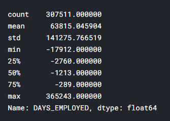
– ( , ) — 1000 !
app_train['DAYS_EMPLOYED'].plot.hist(title = 'Days Employment Histogram');
plt.xlabel('Days Employment');
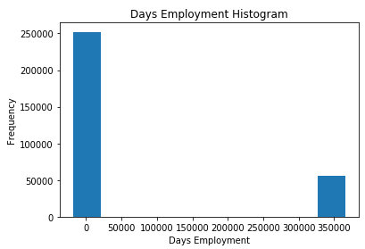
, .
anom = app_train[app_train['DAYS_EMPLOYED'] == 365243]
non_anom = app_train[app_train['DAYS_EMPLOYED'] != 365243]
print('The non-anomalies default on %0.2f%% of loans' % (100 * non_anom['TARGET'].mean()))
print('The anomalies default on %0.2f%% of loans' % (100 * anom['TARGET'].mean()))
print('There are %d anomalous days of employment' % len(anom))
The non-anomalies default on 8.66% of loans
The anomalies default on 5.40% of loans
There are 55374 anomalous days of employment
– , .
. — , . , , , - . , , , . (np.nan), , , .
# ,
app_train['DAYS_EMPLOYED_ANOM'] = app_train["DAYS_EMPLOYED"] == 365243
# nan
app_train['DAYS_EMPLOYED'].replace({365243: np.nan}, inplace = True)
app_train['DAYS_EMPLOYED'].plot.hist(title = 'Days Employment Histogram');
plt.xlabel('Days Employment');

, . , , ( nans , , ). DAYS , , .
: , , . np.nan .
app_test['DAYS_EMPLOYED_ANOM'] = app_test["DAYS_EMPLOYED"] == 365243
app_test["DAYS_EMPLOYED"].replace({365243: np.nan}, inplace = True)
print('There are %d anomalies in the test data out of %d entries' % (app_test["DAYS_EMPLOYED_ANOM"].sum(), len(app_test)))
There are 9274 anomalies in the test data out of 48744 entries
, , EDA. — . , .corr.
.00–0.19 « »
.20-.39 «»
.40–0.59 «»
0,60–0,79 «»
0,80–1,0 « »
#
correlations = app_train.corr()['TARGET'].sort_values()
#
print('Most Positive Correlations:\n', correlations.tail(15))
print('\nMost Negative Correlations:\n', correlations.head(15))
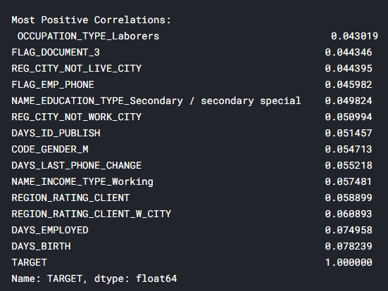
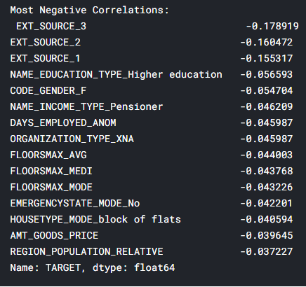
: DAYSBIRTH — ( TARGET, 1). , DAYSBIRTH — . , , , , , (.. == 0). , , .
app_train['DAYS_BIRTH'] = abs(app_train['DAYS_BIRTH'])
app_train['DAYS_BIRTH'].corr(app_train['TARGET'])
-0.07823930830982694
, , , , .
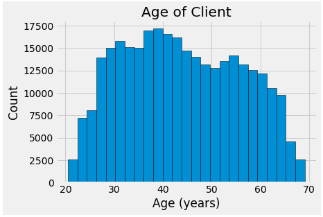
. -, . , x .
plt.style.use('fivethirtyeight')
#
plt.hist(app_train['DAYS_BIRTH'] / 365, edgecolor = 'k', bins = 25)
plt.title('Age of Client'); plt.xlabel('Age (years)'); plt.ylabel('Count');
, , , . , (KDE), . ( , , , ). seaborn kdeplot.
plt.figure(figsize = (10, 8))
sns.kdeplot(app_train.loc[app_train['TARGET'] == 0, 'DAYS_BIRTH'] / 365, label = 'target == 0')
sns.kdeplot(app_train.loc[app_train['TARGET'] == 1, 'DAYS_BIRTH'] / 365, label = 'target == 1')
plt.xlabel('Age (years)'); plt.ylabel('Density'); plt.title('Distribution of Ages');
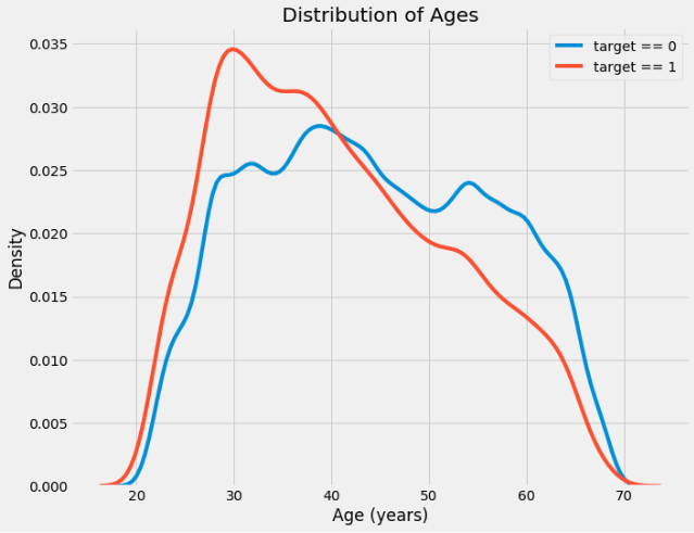
target == 1 . ( -0,07), , , , . : .
, 5 . , .
age_data = app_train[['TARGET', 'DAYS_BIRTH']]
age_data['YEARS_BIRTH'] = age_data['DAYS_BIRTH'] / 365
age_data['YEARS_BINNED'] = pd.cut(age_data['YEARS_BIRTH'], bins = np.linspace(20, 70, num = 11))
age_data.head(10)

#
age_groups = age_data.groupby('YEARS_BINNED').mean()
age_groups

plt.figure(figsize = (8, 8))
plt.bar(age_groups.index.astype(str), 100 * age_groups['TARGET'])
plt.xticks(rotation = 75); plt.xlabel('Age Group (years)'); plt.ylabel('Failure to Repay (%)')
plt.title('Failure to Repay by Age Group');

: . 10% 5% .
: , , . , , , .
: EXTSOURCE1, EXTSOURCE2 EXTSOURCE3. , « ». , , , , , .
.
-, EXT_SOURCE .
ext_data = app_train[['TARGET', 'EXT_SOURCE_1', 'EXT_SOURCE_2', 'EXT_SOURCE_3', 'DAYS_BIRTH']]
ext_data_corrs = ext_data.corr()
ext_data_corrs

plt.figure(figsize = (8, 6))
#
sns.heatmap(ext_data_corrs, cmap = plt.cm.RdYlBu_r, vmin = -0.25, annot = True, vmax = 0.6)
plt.title('Correlation Heatmap');
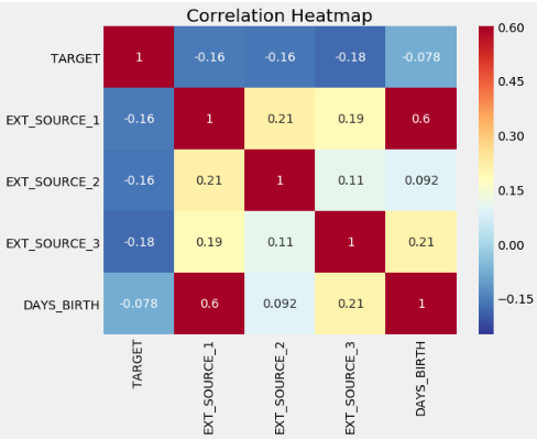
EXT_SOURCE , , EXT_SOURCE . , DAYS_BIRTH EXT_SOURCE_1, , , , .
, . .
plt.figure(figsize = (10, 12))
for i, source in enumerate(['EXT_SOURCE_1', 'EXT_SOURCE_2', 'EXT_SOURCE_3']):
plt.subplot(3, 1, i + 1)
sns.kdeplot(app_train.loc[app_train['TARGET'] == 0, source], label = 'target == 0')
sns.kdeplot(app_train.loc[app_train['TARGET'] == 1, source], label = 'target == 1')
plt.title('Distribution of %s by Target Value' % source)
plt.xlabel('%s' % source); plt.ylabel('Density');
plt.tight_layout(h_pad = 2.5)
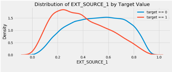
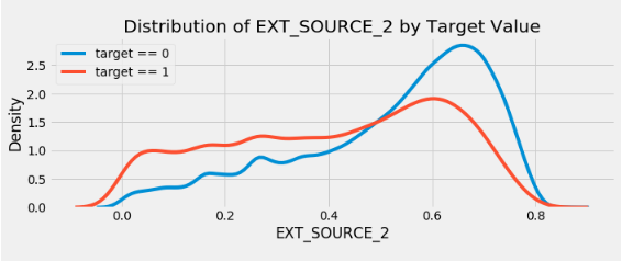
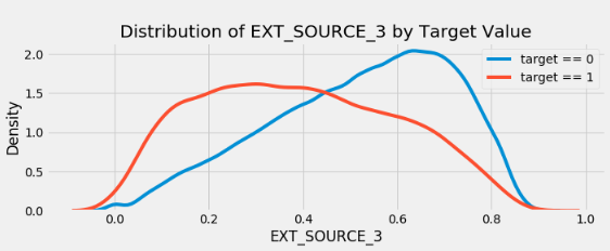
EXT_SOURCE_3 . , . ( ), , , .
EXTSOURCE DAYSBIRTH. – , , . seaborn PairGrid, , 2D .
plot_data = ext_data.drop(columns = ['DAYS_BIRTH']).copy()
plot_data['YEARS_BIRTH'] = age_data['YEARS_BIRTH']
plot_data = plot_data.dropna().loc[:100000, :]
#
def corr_func(x, y, **kwargs):
r = np.corrcoef(x, y)[0][1]
ax = plt.gca()
ax.annotate("r = {:.2f}".format(r),
xy=(.2, .8), xycoords=ax.transAxes,
size = 20)
#
grid = sns.PairGrid(data = plot_data, size = 3, diag_sharey=False,
hue = 'TARGET',
vars = [x for x in list(plot_data.columns) if x != 'TARGET'])
grid.map_upper(plt.scatter, alpha = 0.2)
grid.map_diag(sns.kdeplot)
grid.map_lower(sns.kdeplot, cmap = plt.cm.OrRd_r);
plt.suptitle('Ext Source and Age Features Pairs Plot', size = 32, y = 1.05);
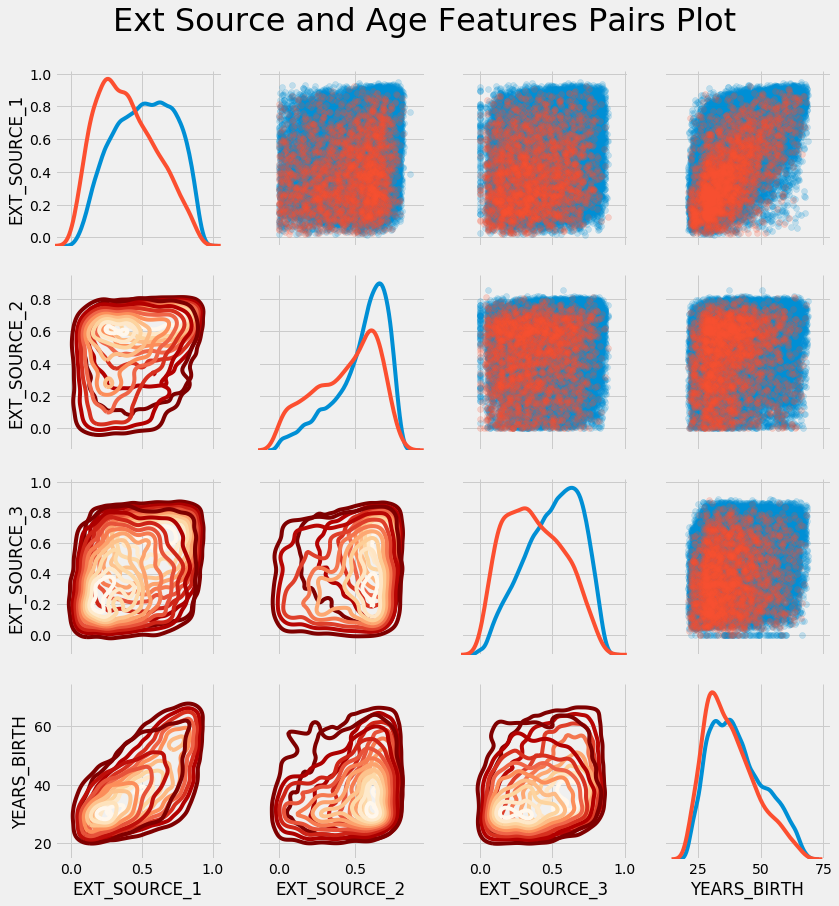
このグラフでは、赤は未返済のローンを示し、青は返済されたローンを示します。データにはさまざまな関係が見られます。EXT_SOURCE_1とYEARS_BIRTHの間には確かに中程度の正の線形関係があり、この特性が年齢に関連している可能性があることを示しています。
これで最初の記事は終わりです。次のパートでは、利用可能なデータに基づいて追加機能を開発する方法について説明し、簡単な機械学習モデルを作成する方法も示します。
記事の作成には、オープンソースの資料が使用されました: source_1、 source_2。