日付と時刻は簡単なオブジェクトではありません。
- 月には異なる日数が含まれます。
- 年はうるう年であり、うるう年ではありません。
- さまざまなタイムゾーンがあります。
- 時間、分、日は異なる数値システムを使用します。
- そして他の多くのニュアンス。
以下は、ドキュメントでめったに強調されないいくつかのポイントの要約と、高速で制御されたコードを書くことを可能にするトリックです。
スマートフォンリーダー向けの非常に短い要約:大量のデータでは、ほんのPOSIXct
数秒しか使用しません。もちろん、すぐに良いでしょう。
これは、以前の一連の出版物の続きです。
日時指定基準
ISO 8601データ要素と交換形式-情報交換-日付と時刻の表現は、日付と時刻に関連するデータの交換を対象とする国際標準です。
時間で作業するための基本的なRメソッド
日付
Sys.Date()
print("-----")
x <- as.Date("2019-01-29") # UTC
print(x)
tz(x)
str(x)
dput(x)
print("-----")
dput(as.Date("1970-01-01")) # ! origin
## [1] "2021-04-29" ## [1] "-----" ## [1] "2019-01-29" ## [1] "UTC" ## Date[1:1], format: "2019-01-29" ## structure(17925, class = "Date") ## [1] "-----" ## structure(0, class = "Date")
初期化中の非標準の日付形式は、特別に指定する必要があります
as.Date("04/20/2011", format = "%m/%d/%Y")
## [1] "2011-04-20"
時間
Rで使用される時間には2つの基本的なタイプがあります:POSIXct
とPOSIXlt
。
外観POSIXct
とPOSIXlt
外観は似ています。そして、内部のもの?
z <- Sys.time()
glue(" ",
"POSIXct - {z}",
"POSIXlt - {as.POSIXlt(z)}", "---", .sep = "\n")
glue(" ",
"POSIXct - {capture.output(dput(z))}",
"POSIXlt - {paste0(capture.output(dput(as.POSIXlt(z))), collapse = '')}",
"---", .sep = "\n")
# /
glue(": {year(z)} \n: {minute(z)}\n: {second(z)}\n---")
## ## POSIXct - 2021-04-29 15:18:04 ## POSIXlt - 2021-04-29 15:18:04 ## --- ## ## POSIXct - structure(1619698684.50764, class = c("POSIXct", "POSIXt")) ## POSIXlt - structure(list(sec = 4.50764489173889, min = 18L, hour = 15L, mday = 29L, mon = 3L, year = 121L, wday = 4L, yday = 118L, isdst = 0L, zone = "MSK", gmtoff = 10800L), class = c("POSIXlt", "POSIXt"), tzone = c("", "MSK", "MSD")) ## --- ## : 2021 ## : 18 ## : 4 ## ---
すぐに、データを扱う真剣な作業(時間とともに10行以上)の場合、POSIXlt
それを悪い夢として忘れていると結論付けます。それは非常識なオーバーヘッドを持つ複雑な構造です。
POSIXct
unixtimestamp, () ( 0 01.01.1970). .
— online unixtimestamp:
- Epoch Unix Time Stamp Converter
- Epoch & Unix Timestamp Conversion Tools
- currentDate / Time in Millisecondsmillis
z <- 1548802400
as.POSIXct(z, origin = "1970-01-01") # local
as.POSIXct(z, origin = "1970-01-01", tz = "UTC") # in UTC
## [1] "2019-01-30 01:53:20 MSK" ## [1] "2019-01-29 22:53:20 UTC"
. . :
- ISO, (ISO 8601-2019);
- - ;
- .
POSIXct
, - . :
x <- ymd_hms("2014-09-24 15:23:10")
x
x + 0.5
x + 0.5 + 0.6
options(digits.secs=5)
x + 0.45756
options(digits.secs=0)
x
## [1] "2014-09-24 15:23:10 UTC" ## [1] "2014-09-24 15:23:10 UTC" ## [1] "2014-09-24 15:23:11 UTC" ## [1] "2014-09-24 15:23:10.45756 UTC" ## [1] "2014-09-24 15:23:10 UTC"
, .
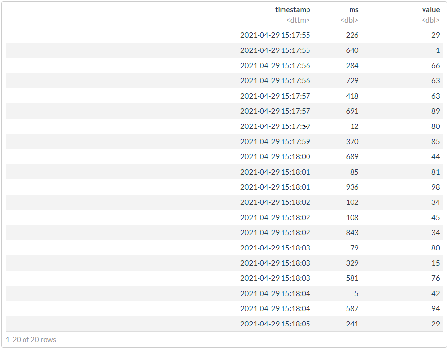
options(digits.secs=5)
# generate data
df <- data.frame(
timestamp = as_datetime(
round(runif(20, min = now() - seconds(10), max = now()), 0),
tz ="Europe/Moscow")) %>%
mutate(ms = round(runif(n(), 0, 999), 0)) %>%
mutate(value = round(runif(n(), 0, 100), 0))
dput(df)
# " "
df %>%
arrange(timestamp, ms)
options(digits.secs=0)
## structure(list(timestamp = structure(c(1619698677, 1619698680, ## 1619698676, 1619698682, 1619698675, 1619698682, 1619698679, 1619698679, ## 1619698684, 1619698683, 1619698684, 1619698677, 1619698682, 1619698683, ## 1619698675, 1619698676, 1619698685, 1619698681, 1619698683, 1619698681 ## ), class = c("POSIXct", "POSIXt"), tzone = "Europe/Moscow"), ## ms = c(418, 689, 729, 108, 226, 843, 12, 370, 5, 581, 587, ## 691, 102, 79, 640, 284, 241, 85, 329, 936), value = c(63, ## 44, 63, 45, 29, 34, 80, 85, 42, 76, 94, 89, 34, 80, 1, 66, ## 29, 81, 15, 98)), class = "data.frame", row.names = c(NA, ## -20L))
# ""
# [magrittr aliases](https://magrittr.tidyverse.org/reference/aliases.html)
df2 <- df %>%
mutate(timestamp = timestamp + ms/1000) %>%
# mutate_at("timestamp", ~`+`(. + ms/1000)) %>%
select(-ms) %>%
df2 %>% arrange(timestamp)

#
dt <- as.data.table(df2)
bench::mark(
naive = dplyr::arrange(df, timestamp, ms),
smart = dplyr::arrange(df2, timestamp),
dt = dt[order(timestamp)],
check = FALSE,
relative = TRUE,
min_iterations = 1000
)
## # A tibble: 3 x 6 ## expression min median `itr/sec` mem_alloc `gc/sec` ## <bch:expr> <dbl> <dbl> <dbl> <dbl> <dbl> ## 1 naive 11.9 11.8 1 1.06 1 ## 2 smart 11.1 11.0 1.06 1 1.06 ## 3 dt 1 1 11.6 494. 1.22
.
data <- c("05102019210003657", "05102019210003757", "05102019210003857")
dmy_hms(stri_c(stri_sub(data, to = 14L), ".", stri_sub(data, from = 15L)), tz = "Europe/Moscow")
#
data2 <- data %>%
sample(10^6, replace = TRUE)
bench::mark(
stri_sub = stri_c(stri_sub(data2, to = 14L), ".", stri_sub(data2, from = 15L)),
stri_replace = stri_replace_first_regex(data2, pattern = "(^.{14})(.*)", replacement = "$1.$2"),
re2_replace = re2_replace(data2, pattern = "(^.{14})(.*)", replacement = "\\1.\\2", parallel = TRUE)
)
## [1] "2019-10-05 21:00:03 MSK" "2019-10-05 21:00:03 MSK" ## [3] "2019-10-05 21:00:03 MSK" ## # A tibble: 3 x 6 ## expression min median `itr/sec` mem_alloc `gc/sec` ## <bch:expr> <bch:tm> <bch:tm> <dbl> <bch:byt> <dbl> ## 1 stri_sub 214ms 222ms 4.10 22.89MB 5.47 ## 2 stri_replace 653ms 653ms 1.53 7.63MB 0 ## 3 re2_replace 409ms 413ms 2.42 15.29MB 1.21
lubridate
x <- ymd(20101215)
print(x)
class(x)
## [1] "2010-12-15" ## [1] "Date"
lubridate
ymd(20101215) == mdy("12/15/10")
## [1] TRUE
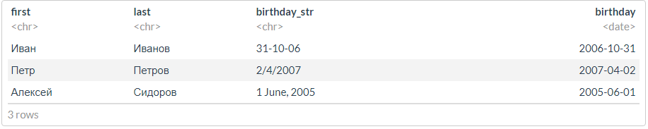
df <- tibble(first = c("", "", ""),
last = c("", "", ""),
birthday_str = c("31-10-06", "2/4/2007", "1 June, 2005")) %>%
mutate(birthday = dmy(birthday_str))
df
, ?
# lubridate
options(lubridate.verbose = TRUE)
# : ..
df <- tibble(time_str = c("08.05.19 12:04:56", "09.05.19 12:05", "12.05.19 23"))
lubridate::dmy_hms(df$time_str, tz = "Europe/Moscow")
print("---------------------")
lubridate::dmy(df$time_str, tz = "Europe/Moscow")
## [1] "2019-05-08 12:04:56 MSK" NA ## [3] NA ## [1] "---------------------" ## [1] NA NA NA
# lubridate
options(lubridate.verbose = TRUE)
lubridate::dmy_hms(df$time_str, truncated = 3, tz = "Europe/Moscow")
## [1] "2019-05-08 12:04:56 MSK" "2019-05-09 12:05:00 MSK" ## [3] "2019-05-12 23:00:00 MSK"
# lubridate
options(lubridate.verbose = TRUE)
# : ..
df <- tibble(date_str = c("08.05.19", "9/5/2019", "2019-05-07"))
#
glimpse(dmy(df$date_str))
print("---------------------")
#
glimpse(ymd(df$date_str))
print("---------------------")
## Date[1:3], format: "2019-05-08" "2019-05-09" NA ## [1] "---------------------" ## Date[1:3], format: "2008-05-19" NA "2019-05-07" ## [1] "---------------------"
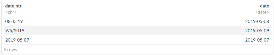
? , , , - .
df %>% mutate(date = dplyr::coalesce(dmy(date_str), ymd(date_str)))
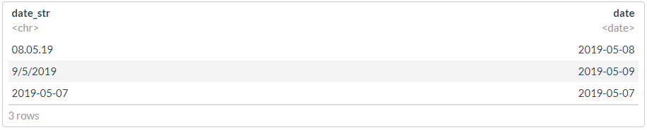
df1 <- df
df1$date <- dmy(df1$date_str)
idx <- is.na(df1$date)
print("---------------------")
idx
df1$date[idx] <- ymd(df1$date_str[idx])
print("---------------------")
df1
## [1] "---------------------" ## [1] FALSE FALSE TRUE ## [1] "---------------------"
"" :
POSIXct
options(lubridate.verbose = FALSE)
date1 <- ymd_hms("2011-09-23-03-45-23")
date2 <- ymd_hms("2011-10-03-21-02-19")
# ?
as.numeric(date2) - as.numeric(date1) # ,
(date2 - date1) %>% dput()
difftime(date2, date1)
difftime(date2, date1, unit="mins")
difftime(date2, date1, unit="secs")
## [1] 926216 ## structure(10.7200925925926, class = "difftime", units = "days") ## Time difference of 10.72009 days ## Time difference of 15436.93 mins ## Time difference of 926216 secs
date1 <- ymd_hms("2019-01-30 00:00:00")
date1
date1 - days(1)
date1 + days(1)
date1 + days(2)
## [1] "2019-01-30 UTC" ## [1] "2019-01-29 UTC" ## [1] "2019-01-31 UTC" ## [1] "2019-02-01 UTC"
—
date1 - months(1)
date1 + months(1) # !!!
## [1] "2018-12-30 UTC" ## [1] NA
. , .
date1 %m-% months(1)
date1 %m+% months(1)
date1 %m+% months(1) %m-% months(1)
## [1] "2018-12-30 UTC" ## [1] "2019-02-28 UTC" ## [1] "2019-01-28 UTC"
date1 <- ymd_hms("2019-01-30 01:00:00")
date1 %T>% print() %>% dput()
with_tz(date1, tzone = "Europe/Moscow") %T>% print() %>% dput()
force_tz(date1, tzone = "Europe/Moscow") %T>% print() %>% dput()
## [1] "2019-01-30 01:00:00 UTC" ## structure(1548810000, class = c("POSIXct", "POSIXt"), tzone = "UTC") ## [1] "2019-01-30 04:00:00 MSK" ## structure(1548810000, class = c("POSIXct", "POSIXt"), tzone = "Europe/Moscow") ## [1] "2019-01-30 01:00:00 MSK" ## structure(1548799200, class = c("POSIXct", "POSIXt"), tzone = "Europe/Moscow")
, , ? , hms
. .
hms_str <- "03:22:14"
as_hms(hms_str)
dput(as_hms(hms_str))
print("-------")
x <- as_hms(hms_str) * 15
x
str(x)
# seconds_to_period(period_to_seconds(x))
seconds_to_period(x) %T>% dput() %>% print()
## 03:22:14 ## structure(12134, units = "secs", class = c("hms", "difftime")) ## [1] "-------" ## Time difference of 182010 secs ## 'difftime' num 182010 ## - attr(*, "units")= chr "secs" ## new("Period", .Data = 30, year = 0, month = 0, day = 2, hour = 2, ## minute = 33) ## [1] "2d 2H 33M 30S"
— . .
( Clickhouse) , , unixtimestamp UTC. , .
:
- . timestamp, , , , , .
- ( ). , , , .
- unixtimestamp UTC , . (!).
- , timestamp. ,
X-1
X+1
, .
, 0.
.
(, ) . , :
- , ;
- ;
- ;
- ( );
- ;
-
double
; - ;
- .
-- ClickHouse
SELECT DISTINCT
store, pos,
timestamp, ms,
concat(toString(store), '-', toString(pos)) AS pos_uid,
toFloat64(timestamp) + (ms / 1000) AS timestamp
flog.info(paste("SQL query:", sql_req))
tic(" CH")
raw_df <- dbGetQuery(conn, stri_encode(sql_req, to = "UTF-8")) %>%
mutate_if(is.character, `Encoding<-`, "UTF-8") %>%
as_tibble() %>%
mutate_at(vars(timestamp), anytime::anytime, tz = "Europe/Moscow") %>%
mutate_at("event", as.factor)
flog.info(capture.output(toc()))
DBI::dbDisconnect(conn)
data.frame
#
df -> as_tibble(_df) %>%
map(pryr::object_size) %>%
unlist() %>%
enframe() %>%
arrange(desc(value)) %>%
mutate_at("value", fs::as_fs_bytes) %>%
mutate(ratio = formattable::percent(value / sum(value), 2)) %>%
add_row(name = "TOTAL", value = sum(.$value))
,
- Epoch & Unix Timestamp Conversion Tools
- currentdate/time in millisecondsmillis
- Functions for working with dates and times
, , , . .
df <- seq.Date(from = as.Date("2021-01-01"),
to = as.Date("2021-05-31"),
by = "2 days") %>%
# sample(20, replace = FALSE) %>%
tibble(date = .)
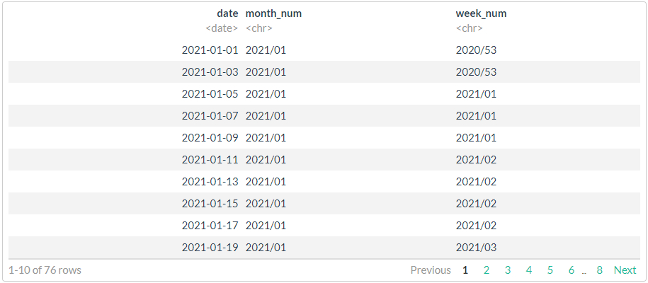
# //
# 1
df %>%
mutate(month_num = stri_c(lubridate::year(date),
sprintf("%02d", lubridate::month(date)),
sep = "/"),
week_num = stri_c(lubridate::isoyear(date),
sprintf("%02d", lubridate::isoweek(date)),
sep = "/")
)
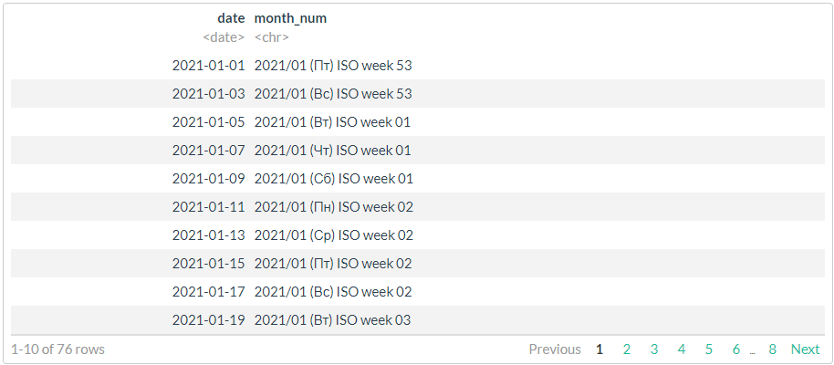
# //
# 2,
# , !!!
df %>%
mutate(month_num = format(date, "%Y/%m (%a) ISO week %V"))
# //
# 3,
# strptime (ISO 8601) ICU
# https://man7.org/linux/man-pages/man3/strptime.3.html
stri_datetime_fstr("%Y/%m (%a) week %V")
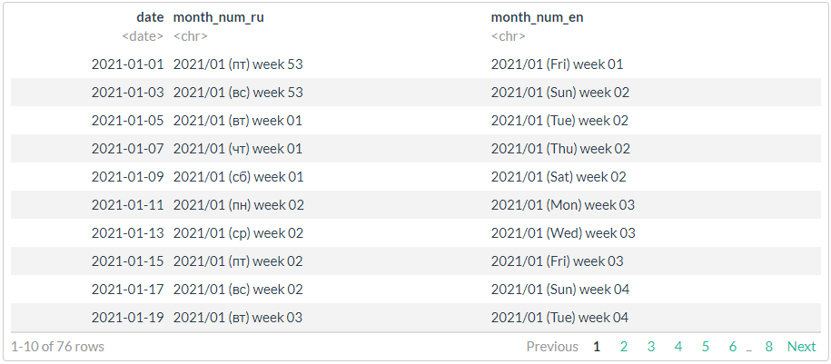
# ggthemes::tableau_color_pal("Tableau 20")(20) %>% scales::show_col()
# , !!!
df %>%
mutate(
month_num_ru = stri_datetime_format(
date, "yyyy'/'MM' ('ccc') week 'ww", locale = "ru", tz = "UTC"),
month_num_en = stri_datetime_format(
date, "yyyy'/'MM' ('ccc') week 'ww", locale = "en", tz = "UTC"))
. .
stri_datetime_format(today(), "LLLL", locale="ru@calendar=Persian")
stri_datetime_format(today(), "LLLL", locale="ru@calendar=Indian")
stri_datetime_format(today(), "LLLL", locale="ru@calendar=Hebrew")
stri_datetime_format(today(), "LLLL", locale="ru@calendar=Islamic")
stri_datetime_format(today(), "LLLL", locale="ru@calendar=Coptic")
stri_datetime_format(today(), "LLLL", locale="ru@calendar=Ethiopic")
stri_datetime_format(today(), "dd MMMM yyyy", locale="ru")
stri_datetime_format(today(), "LLLL d, yyyy", locale="ru")
## [1] "" ## [1] "" ## [1] "" ## [1] "" ## [1] "" ## [1] "" ## [1] "29 2021" ## [1] " 29, 2021"
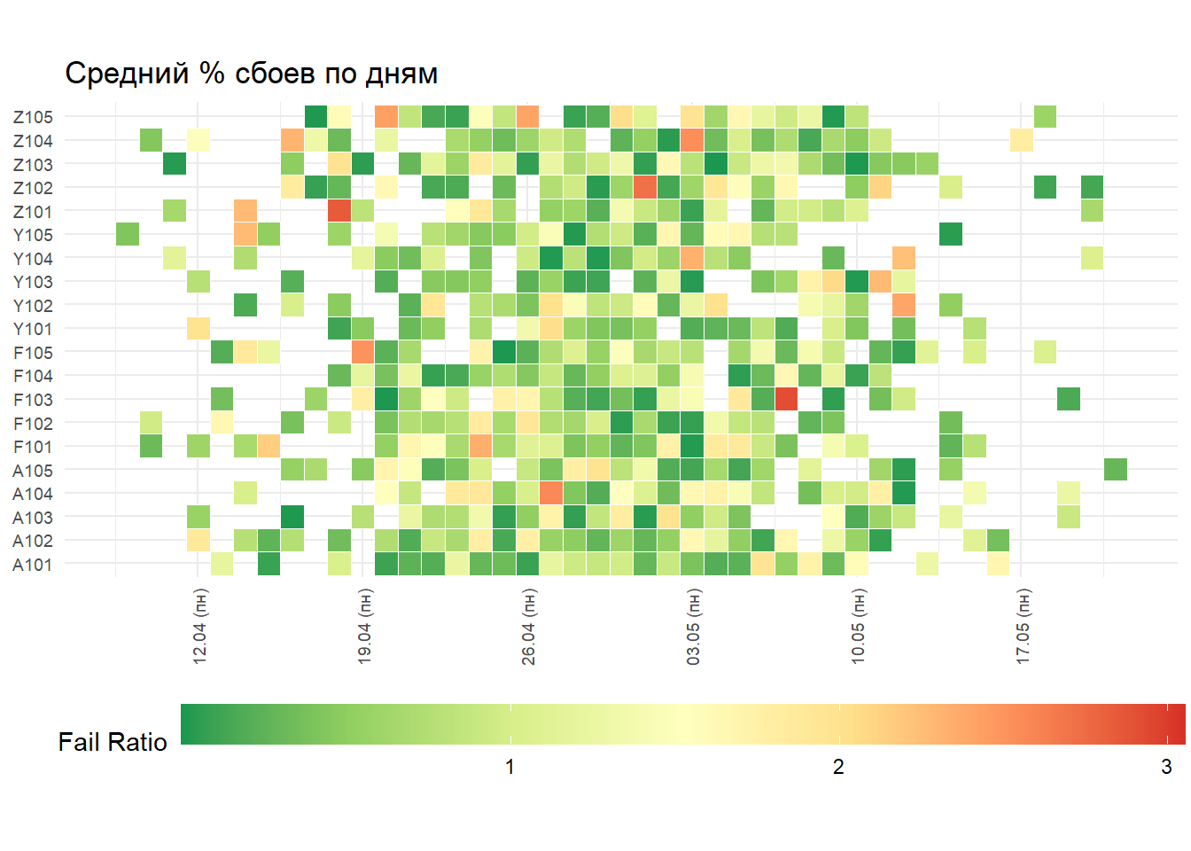
.
#
map_tbl <- tibble(
date = as_date(Sys.time() + rnorm(10^3, mean = 0, sd = 60 * 60 * 24 * 7))) %>%
mutate(store = stri_c(sample(c("A", "F", "Y", "Z"), n(), replace = TRUE),
sample(101:105, n(), replace = TRUE))) %>%
mutate(store_fct = as.factor(store)) %>%
mutate(fail_ratio = abs(rnorm(n(), mean = 0.3, sd = 1)))
my_date_format <- function (format = "dd MMMM yyyy", tz = "Europe/Moscow")
{
scales:::force_all(format, tz)
# stri_datetime_fstr("%d.%m%n%A")
# stri_datetime_fstr("%d.%m (%a)")
function(x) stri_datetime_format(x, format, locale = "ru", tz = tz)
}
# ,
gp <- map_tbl %>%
ggplot(aes(x = date, y = store_fct, fill = fail_ratio)) +
geom_tile(color = "white", size = 0.1) +
# scale_fill_distiller(palette = "RdYlGn", name = "Fail Ratio", label = comma) +
# scale_fill_distiller(palette = "RdYlGn", name = "Fail Ratio", guide = guide_legend(keywidth = unit(4, "cm"))) +
scale_fill_distiller(palette = "RdYlGn", name = "Fail Ratio") +
scale_x_date(breaks = scales::date_breaks("1 week"), labels = my_date_format("dd'.'MM' ('ccc')'")) +
coord_equal() +
labs(x = NULL, y = NULL, title = " % ") +
theme_minimal() +
theme(plot.title = element_text(hjust = 0)) +
theme(axis.ticks = element_blank()) +
theme(axis.text = element_text(size = 7)) +
theme(axis.text.x = element_text(angle = 90, vjust = 0.5)) +
theme(legend.position = "bottom") +
theme(legend.key.width = unit(3, "cm"))
gp
base_df <- tibble(
start = Sys.time() + rnorm(10^3, mean = 0, sd = 60 * 24 * 3)) %>%
mutate(finish = start + rnorm(n(), mean = 100, sd = 60)) %>%
mutate(user_id = sample(as.character(1000:1100), n(), replace = TRUE)) %>%
arrange(user_id, start)
dt <- as.data.table(base_df, key = c("user_id", "start")) %>%
.[, c("start", "finish") := lapply(.SD, as.numeric),
.SDcols = c("start", "finish")]
df <- group_by(base_df, user_id)
bench::mark(
dplyr_v1 = df %>% transmute(delta_t = as.numeric(difftime(finish, start, units = "secs"))) %>% ungroup(),
dplyr_v2 = ungroup(df) %>% transmute(delta_t = as.numeric(difftime(finish, start, units = "secs"))),
dplyr_v3 = dt %>% transmute(delta_t = finish - start),
dt_v1 = dt[, .(delta_t = finish - start), by = user_id],
dt_v2 = dt[, .(delta_t = finish - start)],
check = FALSE # all_equal
)
## # A tibble: 5 x 6 ## expression min median `itr/sec` mem_alloc `gc/sec` ## <bch:expr> <bch:tm> <bch:tm> <dbl> <bch:byt> <dbl> ## 1 dplyr_v1 4.3ms 4.86ms 200. 103.1KB 11.4 ## 2 dplyr_v2 2.17ms 2.46ms 380. 17.9KB 6.24 ## 3 dplyr_v3 1.67ms 1.77ms 527. 29.8KB 8.51 ## 4 dt_v1 410.4us 438.7us 2139. 90.8KB 8.35 ## 5 dt_v2 304.4us 335.3us 2785. 264.6KB 8.38
: //. , , ?
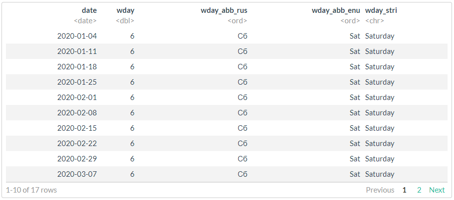
サンプルコード。コードが実行されるマシンのロケールを考慮して、多くの関数が機能することを忘れないでください。また、月がロシア語で印刷されている場合、これは(メソッドを使用しない場合)別のマシンまたは別のOSでの同様の動作を保証するものではありません。
# https://stackoverflow.com/questions/16347731/how-to-change-the-locale-of-r
# https://jangorecki.gitlab.io/data.cube/library/stringi/html/stringi-locale.html
df <- as.Date("2020-01-01") %>%
seq.Date(to = . + months(4), by = "1 day") %>%
tibble(date = .) %>%
mutate(wday = lubridate::wday(date, week_start = 1),
wday_abb_rus = lubridate::wday(date, label = TRUE, week_start = 1),
wday_abb_enu = lubridate::wday(date, label = TRUE, week_start = 1, locale = "English"),
wday_stri = stringi::stri_datetime_format(date, "EEEE", locale = "en"))
#
filter(df, wday == 6)
PSほとんどのテストは一例です。マシン上で実行できます。数値は完全に異なりますが、依存関係と比率の性質はほぼ同じである必要があります。
前の投稿- 「生産的なループでのR対Python」。