ポスト#2のための 初心者は、記述統計、データをグループ化し、正規分布について。このすべての情報は、選挙データのさらなる分析の基礎を築きます。
記述統計
記述統計、または統計は、データを要約および説明するために使用される数値です。私たちが何を意味するのかを説明するために、選挙区の列を見てみましょう。各選挙区の登録有権者の総数が表示されます。
def ex_1_6():
''' ""'''
return load_uk_scrubbed()['Electorate'].count()
650
nan
データセットから空の値()を除外することで列をすでにクリアしているため、前の例では構成要素の総数を返す必要があります。
要約統計量と呼ばれる記述統計量は、一連の数値の特性を測定するためのさまざまなアプローチです。それらはシーケンスを特徴づけるのに役立ち、さらなる分析のためのガイドラインとして機能することができます。一連の数値から計算できる2つの最も基本的な統計(平均と分散)から始めましょう。
平均
データセットを平均化する最も一般的な方法は、平均を取ることです。平均は、実際にはデータ分布の中心を測定するいくつかの方法の1つです。数値級数の平均値は、Pythonで次のように計算されます。
def mean(xs):
''' '''
return sum(xs) / len(xs)
mean
:
def ex_1_7():
''' ""'''
return mean( load_uk_scrubbed()['Electorate'] )
70149.94
, pandas mean, . :
load_uk_scrubbed()['Electorate'].mean()
— . , — , . , , .
def median(xs):
''' '''
n = len(xs)
mid = n // 2
if n % 2 == 1:
return sorted(xs)[mid]
else:
return mean( sorted(xs)[mid-1:][:2] )
:
def ex_1_8():
''' ""'''
return median( load_uk_scrubbed()['Electorate'] )
70813.5
pandas , median
.
, . , , 50, , .
, , 5048, 50.
«» . , , , . :

s2 — , .

, square_deviation
, xs
. mean, .
def variance(xs):
''' ,
n <= 30'''
mu = mean(xs)
n = len(xs)
n = n-1 if n in range(1, 30) else n
square_deviation = lambda x : (x - mu) ** 2
return sum( map(square_deviation, xs) ) / n
Python **
.
, .. , , .. « ». . , «», . , :
def standard_deviation(xs):
''' '''
return sp.sqrt( variance(xs) )
def ex_1_9():
''' ""'''
return standard_deviation( load_uk_scrubbed()['Electorate'] )
7672.77
pandas , var
std
. , , , ddof=0
, , :
load_uk_scrubbed()['Electorate'].std( ddof=0 )
, .. , . 0 1, 0.5 .
:
[10 11 15 21 22.5 28 30]
, 21 . 0.5-. , 0.0 (), 0.25, 0.5, 0.75 1.0 . , . .
. pandas quantile
. .
def ex_1_10():
''' :
xs,
p- '''
q = [0, 1/4, 1/2, 3/4, 1]
return load_uk_scrubbed()['Electorate'].quantile(q=q)
0.00 21780.00
0.25 65929.25
0.50 70813.50
0.75 74948.50
1.00 109922.00
Name: Electorate, dtype: float64
, , . (0.25) (0.75) , . , .
, , (binning). , Counter
( , ) , . , - , (bins).
, . . , , :

15 x, 5 . , , , , — . Python nbin
:
def nbin(n, xs):
''' '''
min_x, max_x = min(xs), max(xs)
range_x = max_x - min_x
fn = lambda x: min( int((abs(x) - min_x) / range_x * n), n-1 )
return map(fn, xs)
, 0-14 5 :
list( nbin(5, range(15)) )
[0, 0, 0, 1, 1, 1, 2, 2, 2, 3, 3, 3, 4, 4, 4]
, , Counter
, . :
def ex_1_11():
'''m 5 '''
series = load_uk_scrubbed()['Electorate']
return Counter( nbin(5, series) )
Counter({2: 450, 3: 171, 1: 26, 0: 2, 4: 1})
(0 4) , — , , , . .
— . , , , , . , .
, , pandas hist
, .
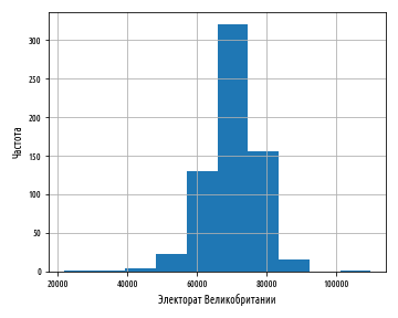
def ex_1_12():
'''
'''
load_uk_scrubbed()['Electorate'].hist()
plt.xlabel(' ')
plt.ylabel('')
plt.show()
:
, , , bins
:
def ex_1_13():
'''
200 '''
load_uk_scrubbed()['Electorate'].hist(bins=200)
plt.xlabel(' ')
plt.ylabel('')
plt.show()
, . , , :
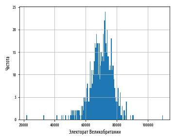
— , , .
def ex_1_14():
'''
20 '''
load_uk_scrubbed()['Electorate'].hist(bins=20)
plt.xlabel(' ')
plt.ylabel('')
plt.show()
20 :

, 20 , , .
, . . — , . , ; , . , , .
, , . .
, , , . , , , .
- , . , , , . , .
: . , . .
. , , , , .
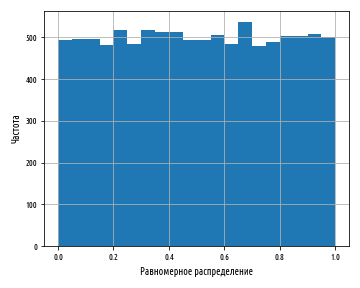
. , scipy stats.uniform.rvs
: . , 0 1 .
def ex_1_15():
'''
'''
xs = stats.uniform.rvs(0, 1, 10000)
pd.Series(xs).hist(bins=20)
plt.xlabel(' ')
plt.ylabel('')
plt.show()
, Series
pandas .
:
, , . , , . , , , , , . .
, , .
def bootstrap(xs, n, replace=True):
'''
n '''
return np.random.choice(xs, (len(xs), n), replace=replace)
def ex_1_16():
''' '''
xs = stats.uniform.rvs(loc=0, scale=1, size=10000)
pd.Series( map(sp.mean, bootstrap(xs, 10)) ).hist(bins=20)
plt.xlabel(' ')
plt.ylabel('')
plt.show()
, :
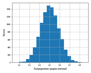
0 1 , . , .
, , , , , .
20- , 1733 . M, , . . , , scipy , :
def ex_1_17():
'''
'''
xs = stats.norm.rvs(loc=0, scale=1, size=10000)
pd.Series(xs).hist(bins=20)
plt.xlabel(' ')
plt.ylabel('')
plt.show()
, sp.random.normal
loc
– , scale
– size
– . :

デフォルトでは、正規分布の平均と標準偏差はそれぞれ0と1です。
この投稿のソースコードの例は、私のGithubリポジトリにあります。すべてのソースデータは、本の著者のリポジトリから取得されます。
「Python、データサイエンス、および選択」投稿シリーズの次のパート3は、比較分析のための分布、それらのプロパティ、およびグラフの生成に専念しています。