「彼女には何も見えません」と私は言って、帽子をシャーロックホームズに返しました。
「いいえ、ワトソン、わかりましたが、見たものを振り返るのに苦労することはありません。
アーサーコナンドイル。青いカーバンクル
ヘンリー・ガーナーの著書 『Clojure for Data Science in Python』のリミックスからの初心者向けの前のシリーズ(最初の投稿はこちら)では、正規分布が何であるかを理解するために、いくつかの数値的および視覚的アプローチが提示されました。平均や標準偏差などのいくつかの記述統計と、それらを使用して大量のデータを簡単に要約する方法について説明しました。
データセットは通常、より大きな母集団または一般的な母集団のサンプルです。この人口が大きすぎて完全に測定できない場合があります。サイズが無限であるため、または直接アクセスできないため、本質的に測定できない場合があります。いずれにせよ、私たちは自由に使えるデータに基づいて結論を出すことを余儀なくされています。
この4投稿シリーズでは、単にサンプルを説明するだけでなく、サンプルが抽出された母集団を説明する方法の統計的意味を見ていきます。サンプリングされたデータから導き出された結論に対する信頼度を詳しく見ていきます。データサイエンスの分野で問題を解決するための堅牢なアプローチの本質を明らかにします。これは、データの研究に科学性をもたらすだけの統計的仮説の検定です。
さらに、プレゼンテーションの過程で、国内統計の用語のドリフトに関連する問題点が強調され、意味があいまいになり、概念が置き換えられることがあります。最終投稿の最後に、次の一連の投稿に賛成または反対票を投じることができます。それまで ...
, AcmeContent, .
AcmeContent
, , , AcmeContent . -, .
, AcmeContent - — . , -. , , - , - , AcmeContent , .
(dwell time)— , - , .
(bounce) — , — .
, , - - - - - - AcmeContent.
, : scipy, pandas matplotlib. pandas Excel, read_excel
. . pandas read_csv
, URL- .
- AcmeContent — - . :
ex_N_M, ex - example (), N - M - . . , .. - . , .
def load_data( fname ):
return pd.read_csv('data/ch02/' + fname, '\t')
def ex_2_1():
return load_data('dwell-times.tsv').head()
( Python Jupyter), , :
|
|
date |
dwell-time |
0 |
2015-01-01T00:03:43Z |
74 |
1 |
2015-01-01T00:32:12Z |
109 |
2 |
2015-01-01T01:52:18Z |
88 |
3 |
2015-01-01T01:54:30Z |
17 |
4 |
2015-01-01T02:09:24Z |
11 |
… |
… |
… |
, .
, dwell-time hist:
def ex_2_2():
load_data('dwell-times.tsv')['dwell-time'].hist(bins=50)
plt.xlabel(' , .')
plt.ylabel('')
plt.show()
:
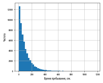
, ; . ( - 0 .). X , , .
, , , Y . , , . , « », . , , .
, , . , 10, , 5 10 4 . , — 30 10 20 . — .
Y logy=True
pandas plot.hist
:
def ex_2_3():
load_data('dwell-times.tsv')['dwell-time'].plot.hist(bins=20, logy=True)
plt.xlabel(' , .')
plt.ylabel(' ')
plt.show()
pandas , 10 . , , -. , - ( , loglog=True
).
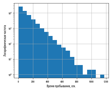
, — . , 10, , , .
— .
( ) , . , , , .
, — . , , . , — , -.
. :
def ex_2_4():
ts = load_data('dwell-times.tsv')['dwell-time']
print(': ', ts.mean())
print(': ', ts.median())
print(' :', ts.std())
: 93.2014074074074
: 64.0
: 93.96972402519819
. , . — .
.
( ). . , -, , , -, . 93 ., , 93 ., - .
, , - 93 . , , - 93 ., 5 . , .
x .
, . , ( ).
64 ., - . 93 . , . 6 . , . .
- . , , . Python, pandas — to_datetime.
, date-time, , , 1- Series
pandas , . , errors='ignore'
, . , mean_dwell_times_by_date
resample
. -, . 'D'
, mean
. , dt.resample('D').mean()
:
def with_parsed_date(df):
''' date date-time'''
df['date'] = pd.to_datetime(df['date'], errors='ignore')
return df
def filter_weekdays(df):
''' '''
return df[df['date'].index.dayofweek < 5] # ..
def mean_dwell_times_by_date(df):
''' '''
df.index = with_parsed_date(df)['date']
return df.resample('D').mean() #
def daily_mean_dwell_times(df):
''' - '''
df.index = with_parsed_date(df)['date']
df = filter_weekdays(df)
return df.resample('D').mean()
, :
def ex_2_5():
df = load_data('dwell-times.tsv')
mus = daily_mean_dwell_times(df)
print(': ', float(means.mean()))
print(': ', float(means.median()))
print(' : ', float(means.std()))
: 90.21042865056198
: 90.13661202185793
: 3.7223429053200348
90.2 . , , . , 3.7 . , , . :
def ex_2_6():
df = load_data('dwell-times.tsv')
daily_mean_dwell_times(df)['dwell-time'].hist(bins=20)
plt.xlabel(' , .')
plt.ylabel('')
plt.show()
:
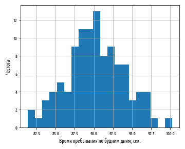
, 90 . 3.7 . , , .. , .
, . , , .
, , .
, - , — , , , . , , .
. , , . ( dropna, , ):
def ex_2_7():
''' '''
df = load_data('dwell-times.tsv')
means = daily_mean_dwell_times(df)['dwell-time'].dropna()
ax = means.hist(bins=20, normed=True)
xs = sorted(means) #
df = pd.DataFrame()
df[0] = xs
df[1] = stats.norm.pdf(xs, means.mean(), means.std())
df.plot(0, 1, linewidth=2, color='r', legend=None, ax=ax)
plt.xlabel(' , .')
plt.ylabel('')
plt.show()
:
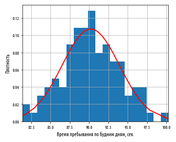
, , , 3.7 . , , 90 . , . 3.7 . — , , .
, (Standard Error, . SE) , , .
— .
, 6 . , , :

σx — , x, n — . , . . , — , :
def variance(xs):
''' () n <= 30'''
x_hat = xs.mean()
n = len(xs)
n = n-1 if n in range(1, 30) else n
square_deviation = lambda x : (x – x_hat) ** 2
return sum( map(square_deviation, xs) ) / n
def standard_deviation(xs):
return sp.sqrt(variance(xs))
def standard_error(xs):
return standard_deviation(xs) / sp.sqrt(len(xs))
:
. , , , .
, , , . , .
次の投稿、投稿#2のトピックは、サンプルと母集団の違い、および信頼区間です。はい、それは信頼区間であり、信頼区間ではありません。