👃🏼 🌅 👴 Pythonで統計に飛び込む。パート3。多くのテストがあります、原則は1つです 👨🏿‍🤝‍👨🏽 🕵🏿 🛩️

良い一日、親愛なるハブラダムとハブラゴスポダ。この記事では、バチスカーフのハッチをできるだけしっかりと閉じ、Pythonエンジンに速度を追加し、日光が実際には浸透しない深さまで統計の深淵に飛び込みます。この深さで、私たちは派手な公式の形で私たちを通り過ぎて浮かぶ多くの種類の統計的検定に遭遇します。最初はそれらがすべて異なって配置されているように見えますが、私たちはこれらすべての奇妙な生き物の主な原動力の底に到達しようとします。

この深さまで潜る前に、私はあなたに何を警告すべきですか？まず、SarahBoslafによる「StatisticsforAll」という本をすでに読んでおり、SciPyライブラリのstatsモジュールの公式ドキュメントにも記載されていると思います。私の次の推測を許してください、しかしあなたはおそらくそこにある膨大な数のテストに少し唖然とし、これが本当に氷山の一角にすぎないことに気付いたときさらに唖然としました。さて、この素晴らしい「思春期」のすべての喜びにまだ遭遇していない場合は、Alexander IvanovichKobzarによる「AppliedMathematicalStatistics。ForEngineersandScientists」という本を入手することをお勧めします。さて、あなたが「主題の中に」いるなら、それでも猫の下を見てください、どうして？事実の提示と解釈は、事実自体よりも重要で興味深い場合があるためです。

, :

import numpy as np
import pandas as pd
from scipy import stats
import matplotlib.pyplot as plt
import seaborn as sns
from pylab import rcParams
sns.set()
rcParams['figure.figsize'] = 10, 6
%config InlineBackend.figure_format = 'svg'
np.random.seed(42)

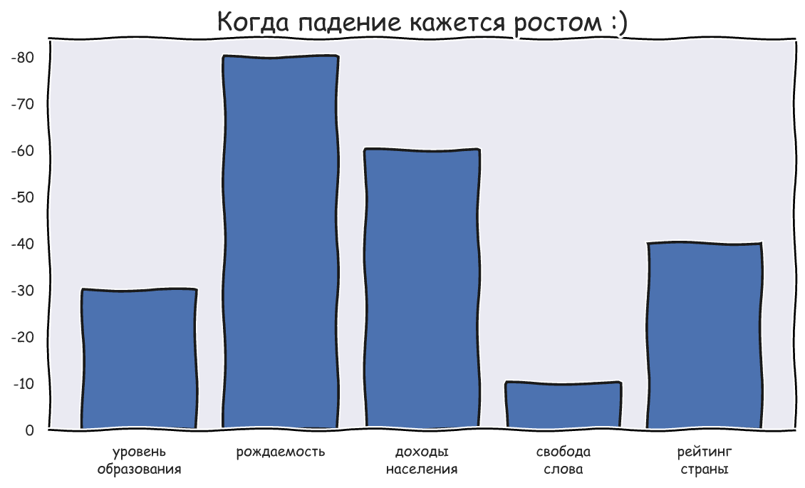
, , . , , - , , . [0; 10] 0 - "", 10 - " ". , :

$x_ {1} = [7.68、\; \; 5.40、\; \; 3.99、\; \; 3.27、\; \; 2.70、\; \; 5.85、\; \; 6.53、\; \; 5.00、\; \; 4.60、\; \; 6.18]$

- , - , - . :

$x_ {2} = [1.33、\; \; 1.66、\; \; 2.76、\; \; 4.56、\; \; 4.75、\; \; 0.70、\; \; 3.13、\; \; 1.96、\; \; 4.60、\; \; 3.69]$

, , , . , . , . , .. . " Pthon - " -.

, , . " , , ", - , , . , : , , .. .. , :

" " ;
" " ;
" " .

, . , , . :

x1 = np.array([7.68,5.40,3.99,3.27,2.70,5.85,6.53,5.00,4.60,6.18])
x2 = np.array([1.33,1.66,2.76,4.56,4.75,0.70,3.13,1.96,4.60,3.69])

fig, ax = plt.subplots()
sns.ecdfplot(x=x1, ax=ax, label=' ')
sns.ecdfplot(x=x2, ax=ax, label='')
ax.legend();

, , ( ), , :

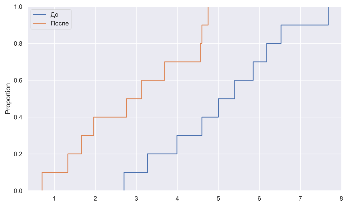
plt.bar(np.arange(10), (x2-x1));

, - . , , , . , :

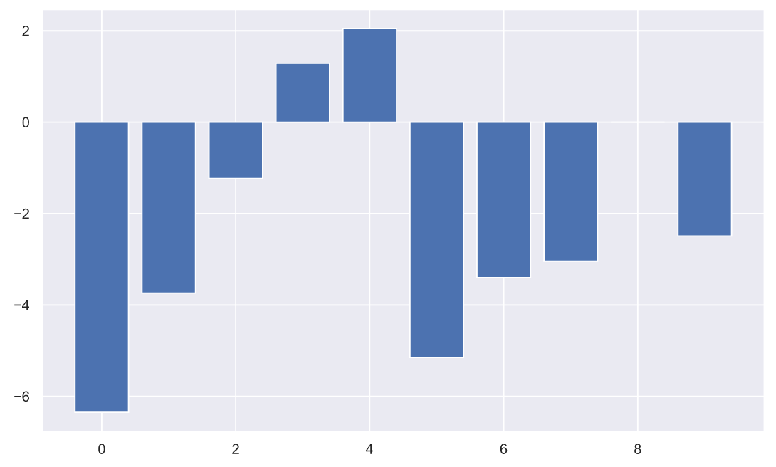
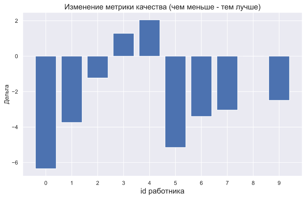
plt.bar(np.arange(10), (x2-x1))
plt.xticks(np.arange(10));
plt.title('   (  -  )',
          fontsize=15)
plt.xlabel('id ', fontsize=15)
plt.ylabel('');

plt.bar(np.arange(10) - 0.2, x1, width=0.4, label='')
plt.bar(np.arange(10) + 0.2, x2, width=0.4, label='')
plt.xticks(np.arange(10))
plt.legend()
plt.title('   (  -  )',
          fontsize=15)
plt.xlabel('id ', fontsize=15)
plt.ylabel('');

, - , , , . , . , , , , . - .

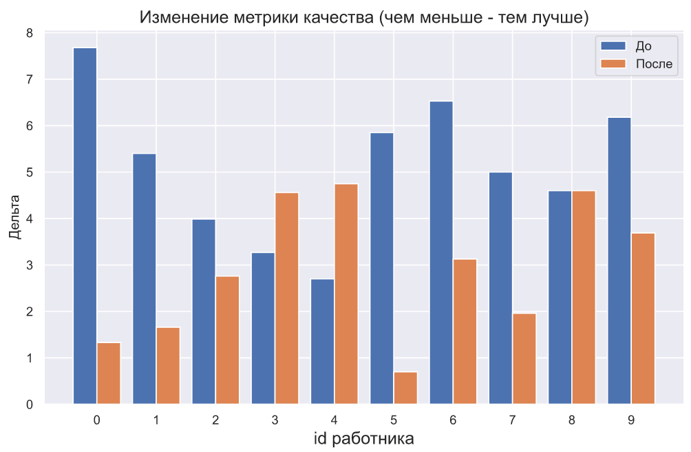
, - t- :

stats.ttest_rel(x2, x1)

Ttest_relResult(statistic=-2.5653968678354184, pvalue=0.03041662395965993)

$\アルファ= 0.05$ c p-value 0.03 , . , . - . ?

print(f'mean(x1) = {x1.mean():.3}')
print(f'mean(x2) = {x2.mean():.3}')
print('-'*15)
print(f'std(x1) = {x1.std(ddof=1):.3}')
print(f'std(x2) = {x2.std(ddof=1):.3}')

mean(x1) = 5.12
mean(x2) = 2.91
---------------
std(x1) = 1.53
std(x2) = 1.47

t- , , (, ), . ? , ? ? , , .. , . , ?

( ) - -. , () , . , - . - , . , , - - . - , .

, t- , , . , . , . , ?

, . 5000 $N（5、1.5 ^ {2}）$ $N（3、1.5 ^ {2}）$ 10 , :

samples = stats.norm.rvs(loc=(5, 3), scale=1.5, size=(5000, 10, 2))
deviations = samples.var(axis=1, ddof=1)
deviations_df = pd.DataFrame(deviations, columns=['s1', 's2'])

sns.histplot(data=deviations_df, element="poly", color='r', fill=False);

, , "" - . :

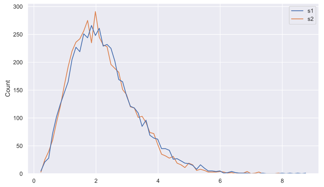
sns.histplot(data=pd.DataFrame(np.std(stats.norm.rvs(loc=(5, 3), scale=1.5, size=(5000,10,2)), axis=1, ddof=1), columns=['s1', 's2']), element="poly", color='r', fill=False);

"" - . - , , :

- ;
;
, .

, - "", "". " ", .. . , , , . , .

, . , , , . : "" . , ", " - , - . , fit():

df1, loc1, scale1 = stats.chi2.fit(deviations_df['s1'], fdf=10)
print(f'df1 = {df1}, loc1 = {loc1:<8.4}, scale1 = {scale1:.3}')

df2, loc2, scale2 = stats.chi2.fit(deviations_df['s2'], fdf=10)
print(f'df2 = {df2}, loc2 = {loc2:<8.4}, scale1 = {scale2:.3}')

df1 = 10, loc1 = -0.1027 , scale1 = 0.238
df2 = 10, loc2 = -0.08352, scale1 = 0.231

fig, ax = plt.subplots()

#     , 
#        0.5   1:
sns.histplot(data=deviations_df['s1'], color='r', element='poly',
             fill=False, stat='density', label='s1', ax=ax)
sns.histplot(data=deviations_df['s2'], color='b', element='poly',
             fill=False, stat='density', label='s2', ax=ax)


chi2_rv1 = stats.chi2(df1, loc1, scale1)
chi2_rv2 = stats.chi2(df2, loc2, scale2)
x = np.linspace(0, 8, 300)
sns.lineplot(x=x, y=chi2_rv1.pdf(x), color='r', label='pdf(s1)', ax=ax)
sns.lineplot(x=x, y=chi2_rv2.pdf(x), color='b', label='pdf(s2)', ax=ax)
ax.set_xticks(np.arange(10))
ax.set_xlabel('s');

- . , , , , , , ( ). . , (""), ("") ("") (""), , , . , , , "" , , .

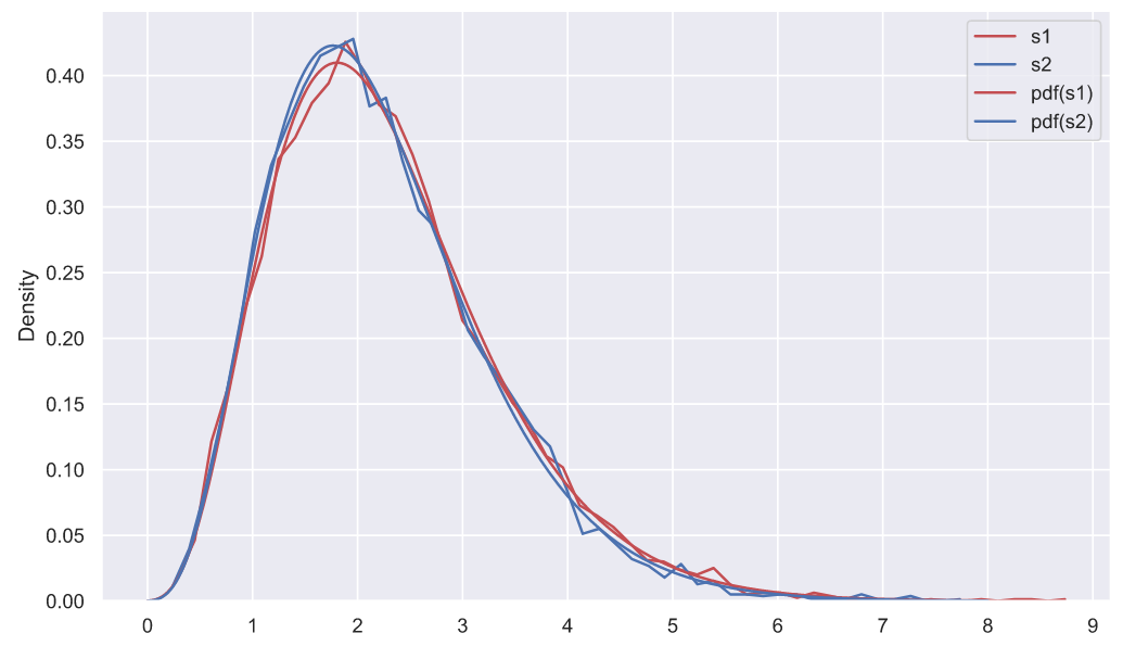
? , , $N（5、1.5 ^ {2}）$ $N（3、1.5 ^ {2}）$ . , . ? , 2, $N（5、1.5 ^ {2}）$ ?

fig, ax = plt.subplots()

var = 2**2
x = np.linspace(0, 10, 300)

sns.lineplot(x=x, y=chi2_rv1.pdf(x), label='pdf(s1)', ax=ax)
ax.vlines(var, 0, chi2_rv1.pdf(var), color='r', lw=2)


ax.fill_between(x[x>var], chi2_rv1.pdf(x[x>var]),
                np.zeros(len(x[x>var])), alpha=0.3, color='b')
ax.hlines(0, x.min(), x.max(), lw=1, color='k')

p = chi2_rv1.sf(var)
ax.set_title(f'$P(s_{1} \geqslant  {var}) = $' + '{:.3}'.format(p))
ax.set_xlabel('s');

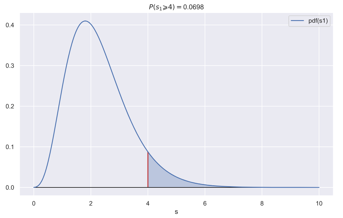
p-value , , , 10 $N（5、1.5 ^ {2}）$ $s \ geqslant 2$ . , $\シグマ$ 1.5. , $\アルファ= 0.05$ , - , .

, - , , 0.1:

fig, ax = plt.subplots()

x = np.linspace(0, 10, 300)
sns.lineplot(x=x, y=chi2_rv1.pdf(x), label='pdf(s1)', ax=ax)

#   :
ci_left, ci_right = chi2_rv1.interval(0.9)
ax.vlines([ci_left, ci_right], 0, 0.5, color='r', lw=2)

x_le_ci_l, x_ge_ci_r = x[x<ci_left], x[x>ci_right]
ax.fill_between(x_le_ci_l, chi2_rv1.pdf(x_le_ci_l),
                np.zeros(len(x_le_ci_l)), alpha=0.3, color='b')
ax.fill_between(x_ge_ci_r, chi2_rv1.pdf(x_ge_ci_r),
                np.zeros(len(x_ge_ci_r)), alpha=0.3, color='b')


ax.set_title(f'P({ci_left:.3} $\geqslant  s_{1} \geqslant$ {ci_right:.3}) = 0.1')


ax.hlines(0, x.min(), x.max(), lw=1, color='k')
ax.set_xlabel('s');

, $\アルファ= 0.1$ , - , , .

? , - . , :

$\ frac {S_ {1、i}} {S_ {2、i}}$

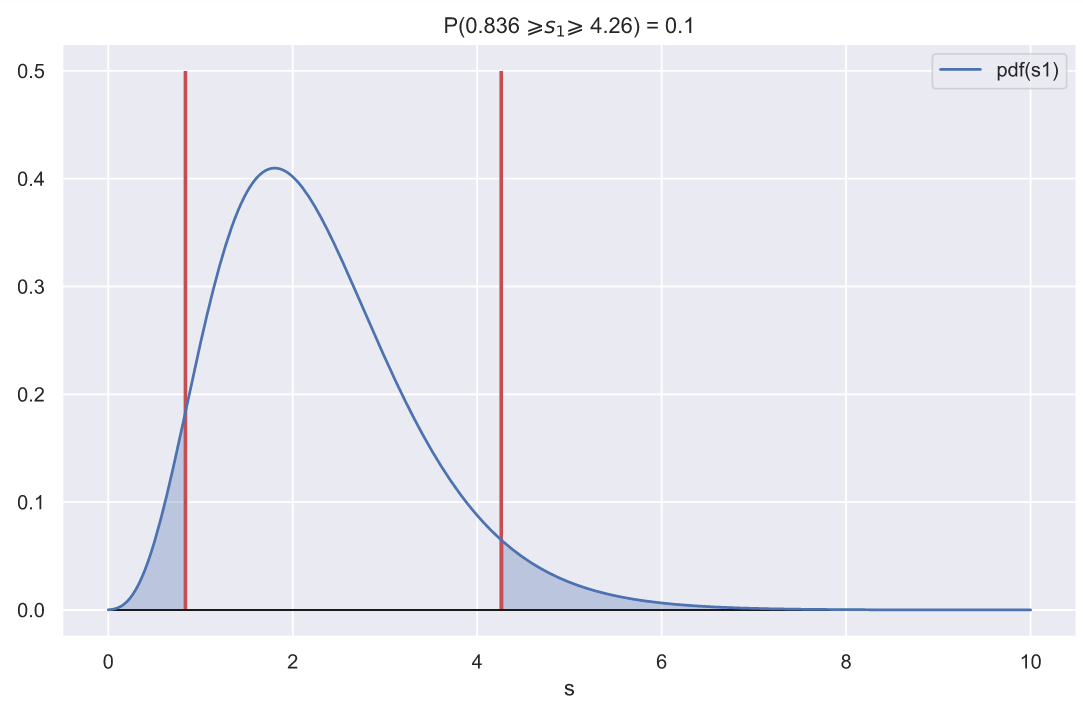
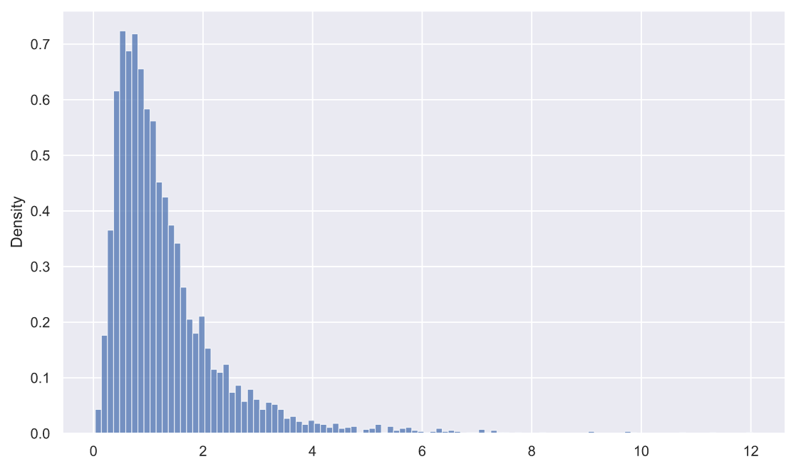
rel_dev = deviations_df['s1'] / deviations_df['s2']
sns.histplot(x=rel_dev, stat='density');

, fit():

dfn, dfd, loc, scale = stats.f.fit(rel_dev, fdfn=10, fdfd=10)
print(f'dfn = {dfn}, dfd = {dfd}, loc2 = {loc2:<8.4}, scale1 = {scale2:.3}')

dfn = 10, dfd = 10, loc2 = -0.08352, scale1 = 0.231

fig, ax = plt.subplots()
rel_dev = deviations_df['s1'] / deviations_df['s2']
sns.histplot(x=rel_dev, stat='density', alpha=0.4)

f_rv = stats.f(dfn, dfd, loc, scale)
x = np.linspace(0, 12, 300)
ax.plot(x, f_rv.pdf(x), color='r')
ax.set_xlim(0, 8);

. , 3, 1, :

fig, ax = plt.subplots()

rel_var = 3
x = np.linspace(0, 8, 300)

sns.lineplot(x=x, y=f_rv.pdf(x), label='pdf(s1)', ax=ax)
ax.vlines(rel_var, 0, f_rv.pdf(rel_var), color='r', lw=2)
ax.fill_between(x[x>rel_var], f_rv.pdf(x[x>rel_var]),
                np.zeros(len(x[x>rel_var])), alpha=0.3, color='b')
ax.hlines(0, x.min(), x.max(), lw=1, color='k')

p = f_rv.sf(var)
ax.set_title(f'$P(s_{1}/s_{2} \geqslant  {rel_var}) = $' + '{:.3}'.format(p))
ax.set_xlabel('s');

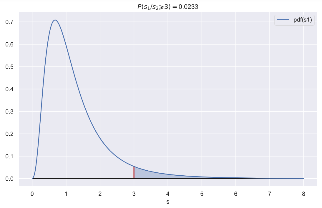
, 10 $N（5、1.5 ^ {2}）$ $N（3、1.5 ^ {2}）$ , , 3, 0.023. , .

np.var(x1, ddof=1) / np.var(x2, ddof=1)

1.083553459313125

. , , . , ? ANOVA? , , , , . f_oneway() ( pvalue, , ):

stats.f_oneway(x1, x2)

F_onewayResult(statistic=10.786061383971454, pvalue=0.0041224402038065235)

? - ?

, f_oneway(), :

$MS _ {\ textrm {bg}} = {\ frac {\ sum _ {j = 1} ^ {m} n_ {j}（M_ {j} -M）^ {2}} {J-1}}$ $MS _ {\ textrm {wg}} = {\ frac {\ sum _ {j = 1} ^ {m} \ sum _ {i = 1} ^ {n_ {j}}（x_ {i、j} -M_ {j}）^ {2}} {NJ}}$

m1, m2, m = *np.mean((x1, x2), axis=1), np.mean((x1, x2))

ms_bg = (10*(m1 - m)**2 + 10*(m2 - m)**2)/(2 - 1)
ms_wg = (np.sum((x1 - m1)**2) + np.sum((x2 - m2)**2))/(20 - 2)
s = ms_bg/ms_wg
p = stats.f.sf(s, dfn=1, dfd=18)
print(f'statistic = {s:.5}, p-value = {p:.5}')

statistic = 10.786, p-value = 0.0041224

$MS _ {\ textrm {bg}}$ (mean square between group) , . , , $MS _ {\ textrm {bg}}$ . $MS _ {\ textrm {wg}}$ (mean square within group) , , . , , , . , - , , . , , $MS _ {\ textrm {bg}}$ $MS _ {\ textrm {wg}}$ :

$\ frac {MS _ {\ textrm {bg}}} {MS _ {\ textrm {bg}}} \ sim F（J-1、N-J）$

N = 10000
samples_1 = stats.norm.rvs(loc=0, scale=1, size=(N, 10))
samples_2 = stats.norm.rvs(loc=0, scale=1, size=(N, 10))

m1 = samples_1.mean(axis=1)
m2 = samples_2.mean(axis=1)
m = np.hstack((samples_1, samples_2)).mean(axis=1)

ms_bg = 10*((m1 - m)**2 + (m2 - m)**2)
ss_1 = np.sum((samples_1 - m1.reshape(N, 1))**2, axis=1)
ss_2 = np.sum((samples_2 - m2.reshape(N, 1))**2, axis=1)
ms_wg = (ss_1 + ss_2)/18

statistics = ms_bg/ms_wg

f, ax = plt.subplots()
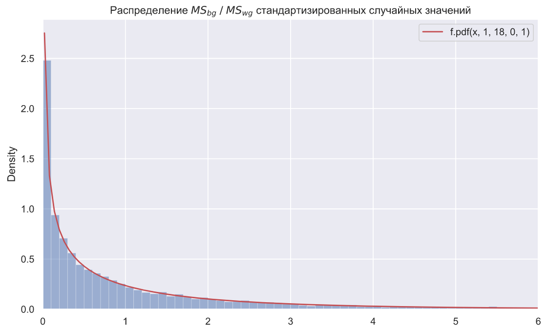
x = np.linspace(0.02, 30, 500)
plt.plot(x, stats.f.pdf(x, dfn=1, dfd=18), color='r', label=f'f.pdf(x, 1, 18, 0, 1)')
plt.legend()
sns.histplot(x=statistics, binwidth=0.1, stat='density', alpha=0.5)
ax.set_xlim(0, 6)
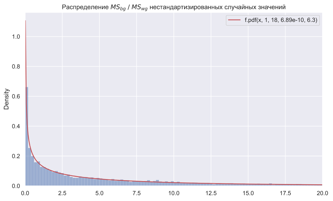
ax.set_title(r' $MS_{bg} \; / \;MS_{wg}$   ');

N = 10000
mu_1 = stats.uniform.rvs(loc=0, scale=5, size=(N, 1))
samples_1 = stats.norm.rvs(loc=mu_1, scale=2, size=(N, 10))
mu_2 = stats.uniform.rvs(loc=0, scale=5, size=(N, 1))
samples_2 = stats.norm.rvs(loc=mu_2, scale=2, size=(N, 10))

m1 = samples_1.mean(axis=1)
m2 = samples_2.mean(axis=1)
m = np.hstack((samples_1, samples_2)).mean(axis=1)

ms_bg = 10*((m1 - m)**2 + (m2 - m)**2)
ss_1 = np.sum((samples_1 - m1.reshape(N, 1))**2, axis=1)
ss_2 = np.sum((samples_2 - m2.reshape(N, 1))**2, axis=1)
ms_wg = (ss_1 + ss_2)/18

statistics = ms_bg/ms_wg

loc, scale = stats.f.fit(statistics, fdfn=1, fdfd=18)[-2:]

f, ax = plt.subplots()
x = np.linspace(0.02, 30, 500)
plt.plot(x, stats.f.pdf(x, dfn=1, dfd=18, loc=loc, scale=scale), color='r', label=f'f.pdf(x, 1, 18, {loc:.3}, {scale:.3})')
plt.legend()
sns.histplot(x=statistics, binwidth=0.2, stat='density', alpha=0.5)
ax.set_xlim(0, 20)
ax.set_title(r' $MS_{bg} \; / \;MS_{wg}$   ');

, SciPy levene(). () , ANOVA, :

stats.levene(x1, x2)

LeveneResult(statistic=0.0047521397921121405, pvalue=0.9458007897725039)

""

, , . , , , , , . , , . : 10000 5 , , , :

N, k = 10000, 5
func = [stats.uniform, stats.norm, stats.laplace]
color = list('gyb')
labels = ['s_uniform', 's_norm', 's_laplace']

for i in range(3):
    ss = np.square(func[i].rvs(size=(N, k))).sum(axis=1)
    sns.histplot(x=ss, stat='density', label=labels[i] + '.pdf(x)',
                 element='step', color=color[i], lw=2, fill=False)
x = np.linspace(0, 25, 300)
plt.plot(x, stats.chi2.pdf(x, df=5), color='r', label='chi2.pdf(x, df=5)')
plt.legend()
plt.xlim(0, 20);

, - , , , "" . , , , - (- - ).

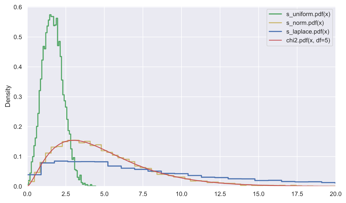
- ANOVA, , "" ? , :

array([0.40572556, 0.67443266, 0.38765587, 0.96540199, 0.57933085])

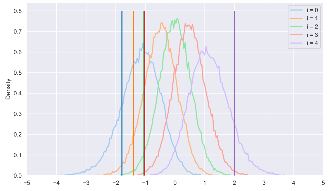
, - . ? 50 5 , , , :

s = np.sort(stats.norm.rvs(size=(50000, 5)), axis=1).T
for i in range(5):
    sns.histplot(x=s[i], stat='density', 
                 label='i = ' + str(i), 
                 element='poly', lw=2, fill=False)
plt.xticks(np.arange(-5, 6))
plt.legend();

, ? , , , . , :

" " ;
;
( );
- , ( );
.

, , , , "" . ?!! , , - :

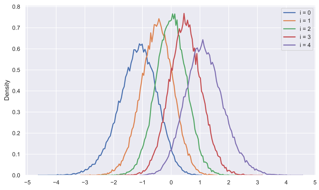
s = np.sort(stats.norm.rvs(size=(50000, 5)), axis=1).T
sample = np.sort(stats.norm.rvs(size=5))
colors = sns.color_palette('tab10', 5)
for i in range(5):
    sns.histplot(x=s[i], stat='density', 
                 label='i = ' + str(i), 
                 element='poly', lw=2, fill=False,
                 color=sns.color_palette('pastel', 5)[i])
    
    plt.vlines(sample[i], 0, 0.8, lw=2,  zorder=10,
               color=sns.color_palette('tab10', 5)[i])
    
plt.xticks(np.arange(-5, 6))
plt.legend();

- :

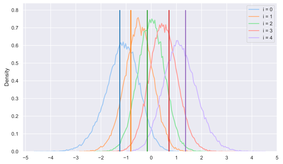
s = np.sort(stats.norm.rvs(size=(50000, 5)), axis=1).T
sample = np.sort(stats.uniform.rvs(loc=-2, scale=4, size=5))
colors = sns.color_palette('tab10', 5)
for i in range(5):
    sns.histplot(x=s[i], stat='density', 
                 label='i = ' + str(i), 
                 element='poly', lw=2, fill=False,
                 color=sns.color_palette('pastel', 5)[i])
    
    plt.vlines(sample[i], 0, 0.8, lw=2,  zorder=10,
               color=sns.color_palette('tab10', 5)[i])
    
plt.xticks(np.arange(-5, 6))
plt.legend();

, - . , , - . : , . , . , . :

stats.ks_1samp(x1, stats.norm.cdf, args=(5, 1.5))

KstestResult(statistic=0.11452966409855592, pvalue=0.9971279018404035)

, p-value, , "" . , , . , , :

x1.sort()
n = len(x1)
ecdf_ge = np.r_[1:n+1]/n
ecdf_le = np.r_[0:n]/n
cdf_teor = stats.norm.cdf(x1, loc=5, scale=1.5)

plt.plot(x1, ecdf_ge, color='b', drawstyle='steps-post', label='ecdf_ge')
plt.plot(x1, cdf_teor, color='r', drawstyle='steps-post', label='cdf_teor')
plt.plot(x1, ecdf_le, color='g', drawstyle='steps-post', label='ecdf_le')
plt.legend();

, .. :

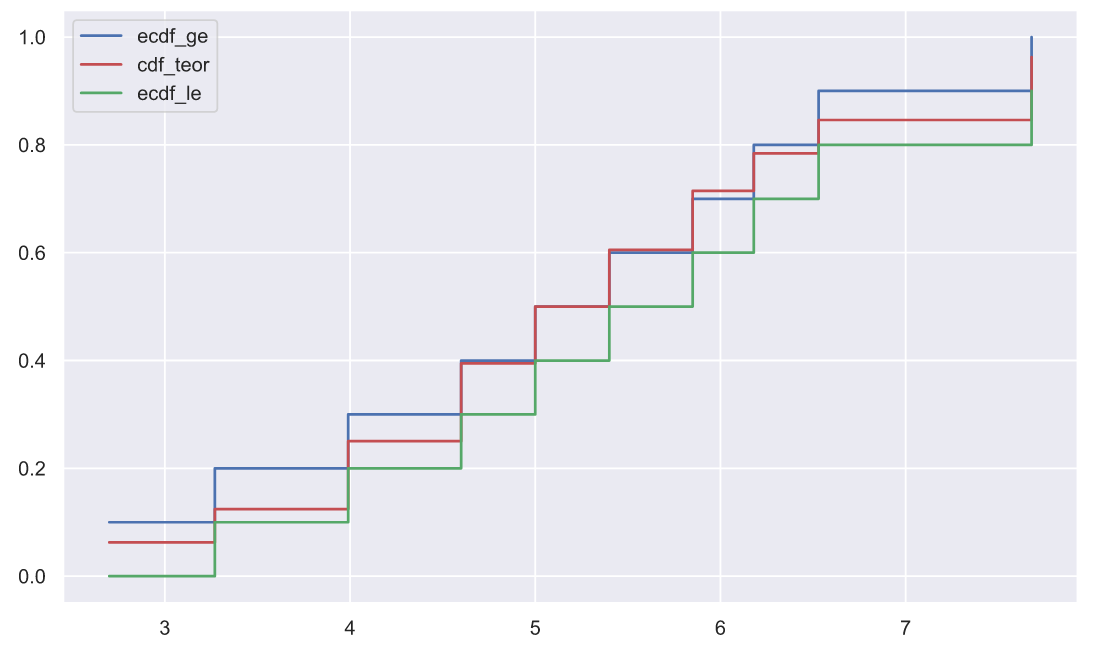
d_plus = ecdf_ge - cdf_teor
d_minus = cdf_teor - ecdf_le
statistic = np.max([d_plus, d_minus])
statistic

0.11452966409855592

( n=5):

x = np.linspace(0, 1, 3000)
plt.plot(x, stats.kstwo.pdf(x, n));

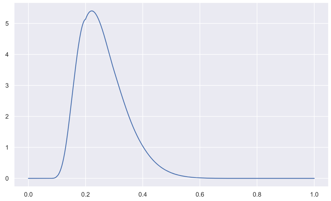
p-value:

pvalue = stats.kstwo.sf(statistic, n)
pvalue

0.9971279018404035

, . , , ecdf_le ( ). , ecdf_le . , "" , seaborn, , .

, , -, , : " ?" , : " , ?" , . , - , , ? , . , - ? , .

科学的および技術的な記事は読むのが簡単ではありませんが、それらを書くことはさらに退屈です。いくつかの複雑なアイデアをシンプルでリラックスした方法で伝えたいと思います。少なくとも少しはできるといいのですが。

それでも、それでも、私たちはダイビングを続けます！エミネムの曲「私の名前は」には、「ウォッカの5分の1を飲んだだけです。あえて運転しますか？（どうぞ）」というお気に入りのセリフがあります。これはダイビング全体に非常に適しています。

いつものように、私はF5を押して、あなたのコメントを楽しみにしています！

Pythonで統計に飛び込む。パート3。多くのテストがあります、原則は1つです

""

More articles: