📴 👩🏾‍🤝‍👨🏻 🛬 Python、相関および回帰：パート4 🚕 👦🏾 🍆

ここで前の投稿を参照してください。

予測

最後に、線形回帰の最も重要なアプリケーションの1つである予測について説明します。身長、性別、生年月日を考慮して、オリンピックの水泳選手の体重を予測するモデルをトレーニングしました。

9回のオリンピック水泳チャンピオンであるマークスピッツは、1972年のオリンピックで7個の金メダルを獲得しました。彼は、1950年に生まれ、ウィキペディアのウェブサイトによると、身長183 cm、体重73kgです。モデルがその重みの観点から何を予測するかを見てみましょう。

私たちの重回帰モデルでは、これらの値を行列形式で提供する必要があります。正しい係数を適用するには、モデルが特徴を学習した順序で各パラメーターを渡す必要があります。バイアスの後、特徴ベクトルには、モデルがトレーニングされたのと同じ単位で、身長、性別、生年月日が含まれている必要があります。

β 行列には、次の各機能の係数が含まれています。

モデルの予測は、各行の係数β と特徴xの積の合計になります。

, β xspitz.

, :

β^Tx — 1 × n n × 1. 1 × 1:

def predict(coefs, x): 
    ''' '''
    return np.matmul(coefs, x.values)

def ex_3_29():
    '''   '''
    df = swimmer_data()
    df['_'] = df[''].map({'': 1, '': 0}).astype(int) 
    df[' '] = df[' '].map(str_to_year)
    X = df[[', ', '_', ' ']] 
    X.insert(0, '', 1.0)
    y = df[''].apply(np.log) 
    beta = linear_model(X, y)
    xspitz = pd.Series([1.0, 183, 1, 1950]) #   
    return np.exp( predict(beta, xspitz) )

84.20713139038605

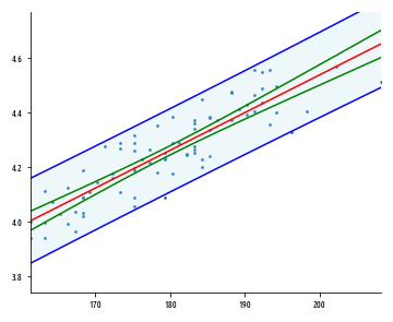
84.21, 84.21 . 73 . , , .

. , , . , , . ŷ , , μ. , , y^.

^{, , , . 95%- – , 95% . , 95%- – , 95%- .}

. , :

ŷ_p — , . t-, n - p, .. . , F-. , , , , , 95%- .

def prediction_interval(x, y, xp):
    '''  '''
    xtx    = np.matmul(x.T, np.asarray(x))
    xtxi   = np.linalg.inv(xtx)  
    xty    = np.matmul(x.T, np.asarray(y)) 
    coefs  = linear_model(x, y) 
    fitted = np.matmul(x, coefs)
    resid  = y - fitted
    rss    = resid.dot(resid)  
    n      = y.shape[0]  # 
    p      = x.shape[1]  # 
    dfe    = n - p 
    mse    = rss / dfe
    se_y   = np.matmul(np.matmul(xp.T, xtxi), xp)
    t_stat = np.sqrt(mse * (1 + se_y))         # t-
    intl   = stats.t.ppf(0.975, dfe) * t_stat   
    yp     = np.matmul(coefs.T, xp)
    return np.array([yp - intl, yp + intl])

t- , .

, se_y

t- t_stat

.

, , :

5 , 95%- . , :

def ex_3_30():
    ''' 
            '''
    df = swimmer_data()
    df['_'] = df[''].map({'': 1, '': 0}).astype(int) 
    df[' '] = df[' '].map(str_to_year)
    X = df[[', ', '_', ' ']] 
    X.insert(0, '', 1.0)
    y = df[''].apply(np.log) 
    xspitz = pd.Series([1.0, 183, 1, 1950])  #  .
    return np.exp( prediction_interval(X, y, xspitz) )

array([72.74964444, 97.46908087])

72.7 97.4 ., 73 ., 95%- . .

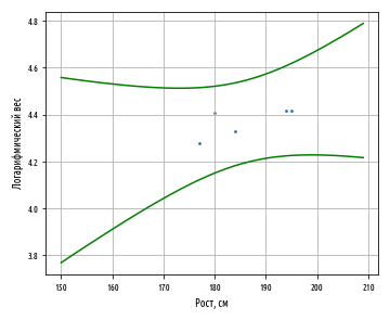
1950 ., 2012 . , , , . .

, . , , . , , . 1979 ., .

, 1972 . 22- 185 . 79 .

^{— .}

, , .

R², , . , .. , , , - .

β :

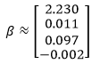
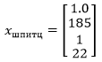
1972 . :

def ex_3_32():
    '''    
        '''
    df = swimmer_data()
    df['_'] = df[''].map({'': 1, '': 0}).astype(int) 
    X = df[[', ', '_', '']] 
    X.insert(0, '', 1.0)
    y = df[''].apply(np.log) 

    beta = linear_model(X, y)
    #    
    xspitz = pd.Series([1.0, 185, 1, 22]) 
    return np.exp( predict(beta, xspitz) )

78.46882772630318

78.47, .. 78.47 . , 79 .

Github. .

, . , r R² R̅². , ρ .

, Python. , pandas numpy . β, , . , .

Python、相関および回帰：パート4

予測

More articles: